Blog By Alexander

0%

Alexander Ezharjan


Introduction

This reference book is mainly to discuss the detailed knowledge of basic computer graphics based on the soft renderer project called Render Engine, which is a tiny graphical rendering engine developed via pure C++ without any third-party-libraries included.


The content of this book is separated into many parts so that we are able to to have a deeper view into each section.

The first section is this Introduction it self.

The second section is to discuss the mathematical basis for computer graphics. The advanced part as well as those part that have tight relation with the physics is not included, as we are just learning the basic knowledge of computer graphics, not the advanced ones.

The third section is to discuss the inside of render pipeline, which is a significant aspect in the study of computer graphics.

The forth section is to discuss the basic unit used in render engine — Vertex. A vertex stores lots of information including position, tex-coord, normal etc,.


In order to relate the CG knowledge into the application, we have to apply the theory into reality by programing, With this notes, however, the co-related project demands the basics for C++ programming. But if you take a look at the project code, you will notice that the application of the programming language is really in basic way, as too many properties of C++ is not utilized at all. Only some of the basic data structures and methods of the STL is used to make the code more accessible as well as to facilitate the project. Note that any other programing languages are OK to apply the theory I clarified in this book.


Math Basis

Math is needed as the basic tool for every field of science. As the base of the computer science, I myself also regard it as the base of computer graphics, for many algorithms can not escape from the use of math. I separated it as a single chapter so as to mention its importance as well as to show you the utility of math in computer graphics.

In math, we have vectors, matrices, coordinates and more. These are all used in computer graphics. If you have ever used OpenGL or any other libraries, you’ll notice that the math is actually provided as basic APIs and using them is quite simple. But if you are writing the CPU based renderer like I have done in this project, you ought to know the inner activities that these APIs are conducting. Here I am going to show you some of the APIs that I wrote:

1
2
3
4
5
6
7
8
9
10
11
12
13
14
15
16
17
18
19
20
21
22
23
24
25
26
27
28
29
30
31
32
33
34
35
36
37
38
39
40
41
42
43
44
45
46
47
48
49
50
51
52
53
54
55
56
57
58
59
60
61
62
63
64
65
66
67
68
69
70
71
72
73
74
75
76
77
78
79
80
81
82
83
84
85
86
87
88
89
90
91
92
93
94
95
96
97
98
99
100
101
102
103
104
105
106
107
108
109
110
111
112
113
114
115
116
117
118
119
120
121
122
123
124
125
126
127
128
129
130
131
132
133
134
135
136
137
138
139
140
141
142
143
144
145
146
147
148
149
150
151
152
153
154
155
156
157
158
159
160
161
162
163
164
165
166
   float RadToDegree(const float& rad) {
return (rad * 180.f / MATH_PI);
}

float DegreeToRad(const float& degree) {
return (degree * MATH_PI / 180.f);
}

float LinearInerpolate(const float& x1, const float& x2, const float& t)
{
return x1 + (x2 - x1) * t; // formula of linear interpolation
}


float Lerp(const float a, const float b, const float t)
{
if (t <= 0.f)
{
return a;
}
else if (t >= 1.f)
{
return b;
}
else
{
return b * t + (1.f - t) * a;
}
}

Vector4 Lerp(const Vector4& a, const Vector4& b, float t)
{
Vector4 result(
Lerp(a.getX(), b.getX(), t),
Lerp(a.getY(), b.getY(), t),
Lerp(a.getZ(), b.getZ(), t),
Lerp(a.getW(), b.getW(), t)
);
return result;
}

Colour Lerp(const Colour& a, const Colour& b, float t)
{
Colour result;
result.r = Lerp(a.r, b.r, t);
result.g = Lerp(a.g, b.g, t);
result.b = Lerp(a.b, b.b, t);
return result;
}


float Clamp(const float& param, const float& min, const float& max)
{
if (param <= min)
return min;
else if (param >= max)
return max;

return param;

// optimized way below
//return ((param < min) ? min : ((param > max) ? max : param));
}

void CLAMP(float& param, const float& min, const float& max)
{
if (param <= min)
param = min;
else if (param >= max)
param = max;
}

void ColorInterpolation(Vertex & s1, Vertex & s3, Vertex & s4)
{
s4.color.r = (s4.pos.getY() - s1.pos.getY()) *(s3.color.r - s1.color.r) / (s3.pos.getY() - s1.pos.getY()) + s1.color.r;
s4.color.g = (s4.pos.getY() - s1.pos.getY()) *(s3.color.g - s1.color.g) / (s3.pos.getY() - s1.pos.getY()) + s1.color.g;
s4.color.b = (s4.pos.getY() - s1.pos.getY()) *(s3.color.b - s1.color.b) / (s3.pos.getY() - s1.pos.getY()) + s1.color.b;
}

bool isPrimeNumber(const int& num)
{
for (size_t i = 2; i < num; i++)
{
if (num % i == 0)
{
return false;
}
}
return true;
}


float StringToNum(const std::string & str)
{
std::istringstream iss(str);
int num;
iss >> num;
return (float)num;
}


int CharToNum(const char& c)
{
return atoi(&c);
}

float Sigmoid(const float x)
{
return (1 / 1 + exp(-x));
}

unsigned char FloatToByte(const float x)
{
return unsigned char((int)(x * 255.f) % 256);
}

float MapTo0_255f(const float x)
{
float result = Clamp(x, 0.f, 0.999999f) * 255.f; // never dropping value ranging 0~1
if (result - EPSILON >= 1.f)
result = floorf(Clamp(x, 0.f, 0.999999f) * 256.f);
return result;
}

float GetGrayScaleViaGamaCorrection(const Colour& valueToBeCorrected)
{
float numerator = powf(MapTo0_255f(valueToBeCorrected.r), 2.2f) + powf((1.5f*MapTo0_255f(valueToBeCorrected.g)), 2.2f) + powf((0.6f*MapTo0_255f(valueToBeCorrected.b)), 2.2f);
float denominator = 1.f + powf(1.5f, 2.2f) + powf(0.6f, 2.2f);
float result = powf((numerator / denominator), 1.f / 2.2f);
return result;
}

Colour GetGrayScaleViaGamaCorrection(const float sameRGBValue)
{
float numerator = powf(MapTo0_255f(sameRGBValue), 2.2f) + powf((1.5f*MapTo0_255f(sameRGBValue)), 2.2f) + powf((0.6f*MapTo0_255f(sameRGBValue)), 2.2f);
float denominator = 1.f + powf(1.5f, 2.2f) + powf(0.6f, 2.2f);
float result = powf((numerator / denominator), 1.f / 2.2f);
return Colour(result, result, result);
}

float GetBrightnessViaGamaCorrection(const Colour & valueToBeCorrected)
{
float numerator = powf(valueToBeCorrected.r, 2.2f) + powf((1.5f*valueToBeCorrected.g), 2.2f) + powf((0.6f*valueToBeCorrected.b), 2.2f);
float denominator = 1.f + powf(1.5f, 2.2f) + powf(0.6f, 2.2f);
float result = powf((numerator / denominator), 1.f / 2.2f);
return result;
}

Colour GetBrightnessViaGamaCorrection(const float sameRGBValue)
{
float numerator = powf(sameRGBValue, 2.2f) + powf((1.5f*sameRGBValue), 2.2f) + powf((0.6f*sameRGBValue), 2.2f);
float denominator = 1.f + powf(1.5f, 2.2f) + powf(0.6f, 2.2f);
float result = powf((numerator / denominator), 1.f / 2.2f);
return Colour(result, result, result);
}


Vector4 Vector4DotMatrix4f(const Vector4 & vec4, const Matrix4f & m4f)
{
Vector4 result;
result.setX(vec4.getX() * m4f.matrix[0][0] + vec4.getY() * m4f.matrix[1][0] + vec4.getZ() * m4f.matrix[2][0] + vec4.getW() * m4f.matrix[3][0]);
result.setY(vec4.getX() * m4f.matrix[0][1] + vec4.getY() * m4f.matrix[1][1] + vec4.getZ() * m4f.matrix[2][1] + vec4.getW() * m4f.matrix[3][1]);
result.setZ(vec4.getX() * m4f.matrix[0][2] + vec4.getY() * m4f.matrix[1][2] + vec4.getZ() * m4f.matrix[2][2] + vec4.getW() * m4f.matrix[3][2]);
result.setW(vec4.getX() * m4f.matrix[0][3] + vec4.getY() * m4f.matrix[1][3] + vec4.getZ() * m4f.matrix[2][3] + vec4.getW() * m4f.matrix[3][3]);
return result;
}

Actually, some of the APIs can be directly gain from STL or ‘math.h’ while you’re using C++, such as the function ‘RadToDegree’ above can also be found in Lua’s inner math library, but writing them done is a way to apply what you have learnt into practice. Hope you can directly use the ones that the inner libraries provide rather than writing them by yourself so as to avoid mistakes and prevent the performance of your application from being lowered.

Here are some of the APIs when defining Vectors:

1
2
3
4
5
6
7
8
9
10
11
12
13
14
15
16
17
18
19
20
21
22
23
24
25
26
27
28
29
30
31
32
33
34
35
36
37
38
39
40
41
42
43
44
45
46
47
48
49
50
51
52
53
54
55
56
57
58
59
60
61
62
63
64
65
66
67
68
69
70
71
72
73
74
75
76
77
78
79
80
81
82
83
84
85
86
87
88
89
90
91
92
93
94
95
96
97
98
99
100
101
102
103
104
105
106
107
108
109
110
111
112
113
114
115
116
117
118
119
120
121
122
123
124
125
126
127
128
129
130
131
132
133
134
135
136
137
138
139
140
141
142
143
144
145
146
147
148
149
150
151
152
153
154
155
156
157
158
159
160
161
162
163
164
165
166
167
168
169
170
171
172
173
174
175
176
177
178
179
180
181
182
183
184
185
186
187
188
189
190
191
192
193
194
195
196
197
198
199
200
201
202
203
204
205
206
207
208
209
210
211
212
213
214
215
216
217
218
219
220
221
222
223
224
225
226
227
228
229
230
231
232
233
234
235
236
237
238
239
240
241
242
243
244
245
246
247
248
249
250
251
252
253
254
255
256
257
258
259
260
261
262
263
264
265
266
267
268
269
270
271
272
273
274
275
276
277
278
279

/************************************************************************/
/* Vector2 */
/************************************************************************/
void Vector2::operator=(const Vector2 & right)
{
this->setX(right.getX());
this->setY(right.getY());
}

Vector2 Vector2::operator+(const Vector2& right) const
{
Vector2 result(this->getX() + right.getX(), this->getY() + right.getY());
return result;
}

Vector2 Vector2::operator-(const Vector2& right) const
{
Vector2 result(this->getX() - right.getX(), this->getY() - right.getY());
return result;
}

template<typename T>
Vector2 Vector2::operator*(const T& k) const
{
Vector2 result(this->getX() * k, this->getY() * k);
return result;
}

Vector2 Vector2::operator /(const float& k) const
{
if (k == 0.f || abs(k - 0.f) < EPSILON) {
return Vector2();
}
float reciprocalK = 1 / k;
Vector2 result(this->getX()*reciprocalK, this->getY()*reciprocalK);
return result;
}

float Vector2::operator*(const Vector2& right) const
{
return (this->getX() * right.getX() + this->getY() * right.getY());
}

void Vector2::swap(Vector2 & vecA, Vector2 & vecB)
{
if (vecA == vecB)return;
Vector2 tmp(vecA.getX(), vecA.getY());
vecA = vecB;
vecB = tmp;
}

float Vector2::getLength()
{
return sqrtf(powf(this->getX(), 2) + powf(this->getY(), 2));
}


/************************************************************************/
/* Vector3 */
/************************************************************************/
bool Vector3::operator==(const float right) const
{
bool xIsEqual = fabsf(this->getX() - right) <= EPSILON;
bool yIsEqual = fabsf(this->getY() - right) <= EPSILON;
bool zIsEqual = fabsf(this->getZ() - right) <= EPSILON;
return (xIsEqual && yIsEqual && zIsEqual);
}

bool Vector3::operator==(const Vector3 & right) const
{
bool xIsEqual = fabsf(this->getX() - right.getX()) <= EPSILON;
bool yIsEqual = fabsf(this->getY() - right.getY()) <= EPSILON;
bool zIsEqual = fabsf(this->getZ() - right.getZ()) <= EPSILON;
return (xIsEqual && yIsEqual && zIsEqual);
}

Vector3 Vector3::operator+(const Vector3 & right) const
{
Vector3 result(this->getX() + right.getX(), this->getY() + right.getY(), this->getZ() + right.getZ());
return result;
}

Vector3 Vector3::operator-(const Vector3 & right) const
{
Vector3 result(this->getX() - right.getX(), this->getY() - right.getY(), this->getZ() - right.getZ());
return result;
}

Vector3 Vector3::operator*(const float k) const
{
Vector3 result(this->getX() * k, this->getY() * k, this->getZ() * k);
return result;
}


float Vector3::operator*(const Vector3 & right) const
{
return (this->getX()*right.getX() + this->getY()*right.getY() + this->getZ()*right.getZ());
}

template<typename T>
Vector3 Vector3::operator*(const T& right) const
{
Vector3 result(
this->getX()*right.matrix[0][0] + this->getY()*right.matrix[0][1] + this->getZ() * right.matrix[0][2],
this->getY()*right.matrix[1][0] + this->getY()*right.matrix[1][1] + this->getZ() * right.matrix[1][2],
this->getZ()*right.matrix[2][0] + this->getY()*right.matrix[2][1] + this->getZ() * right.matrix[2][2]);
return result;
}

Vector3 Vector3::operator^(const Vector3 & right) const
{
Vector3 result;
result.setX(this->getY() * right.getZ() - this->getZ() * right.getY());
result.setY(this->getZ() * right.getX() - this->getX() * right.getZ());
result.setZ(this->getX() * right.getY() - this->getY() * right.getX());
return result;
}

void Vector3::Normalize()
{
float length = sqrtf(powf(this->getX(), 2) + powf(this->getY(), 2) + powf(this->getZ(), 2));
this->setX(this->getX() / length);
this->setY(this->getY() / length);
this->setZ(this->getZ() / length);
}

Vector3 Vector3::Normalize(const Vector3& vecToBeNormalized)
{
Vector3 result;
float length = sqrtf(powf(vecToBeNormalized.getX(), 2) + powf(vecToBeNormalized.getY(), 2) + powf(vecToBeNormalized.getZ(), 2));
result.setX(vecToBeNormalized.getX() / length);
result.setY(vecToBeNormalized.getY() / length);
result.setZ(vecToBeNormalized.getZ() / length);
return result;
}

float Vector3::getLength()
{
return sqrtf(powf(this->getX(), 2) + powf(this->getY(), 2) + powf(this->getZ(), 2));
}


/************************************************************************/
/* Vector4 */
/************************************************************************/
bool Vector4::operator==(float right) const
{
bool xIsEqual = fabsf(this->getX() - right) <= EPSILON;
bool yIsEqual = fabsf(this->getY() - right) <= EPSILON;
bool zIsEqual = fabsf(this->getZ() - right) <= EPSILON;
bool wIsEqual = fabsf(this->getW() - right) <= EPSILON;
return (xIsEqual && yIsEqual && zIsEqual && wIsEqual);
}

bool Vector4::operator==(const Vector4 & right) const
{
bool xIsEqual = fabsf(this->getX() - right.getX()) <= EPSILON;
bool yIsEqual = fabsf(this->getY() - right.getY()) <= EPSILON;
bool zIsEqual = fabsf(this->getZ() - right.getZ()) <= EPSILON;
bool wIsEqual = fabsf(this->getW() - right.getW()) <= EPSILON;
return (xIsEqual && yIsEqual && zIsEqual && wIsEqual);
}

bool Vector4::operator!=(const Vector4 & right) const
{
bool xIsInequal = fabsf(this->getX() - right.getX()) > EPSILON;
bool yIsInequal = fabsf(this->getY() - right.getY()) > EPSILON;
bool zIsInequal = fabsf(this->getZ() - right.getZ()) > EPSILON;
bool wIsInequal = fabsf(this->getW() - right.getW()) > EPSILON;
return (xIsInequal || yIsInequal || zIsInequal || wIsInequal);
}

Vector4 Vector4::operator +(const Vector4 & right) const
{
Vector4 result(this->getX() + right.getX(), this->getY() + right.getY(), this->getZ() + right.getZ(), this->getW() + right.getW());
return result;
}

Vector4 Vector4::operator-(const Vector4 & right) const
{
Vector4 result(this->getX() - right.getX(), this->getY() - right.getY(), this->getZ() - right.getZ(), this->getW() - right.getW());
return result;
}

Vector4 Vector4::operator*(const float k) const
{
Vector4 result(this->getX()*k, this->getY()*k, this->getZ() *k, this->getW() *k);
return result;
}

Vector4 Vector4::operator/(const float k) const
{
float reciprocalK = 1 / k;
Vector4 result(this->getX()*reciprocalK, this->getY()*reciprocalK, this->getZ() *reciprocalK, this->getW() *reciprocalK);
return result;
}

float Vector4::operator *(const Vector4 & right) const
{
return this->getX()*right.getX() + this->getY()*right.getY() + this->getZ()*right.getZ() + this->getW()*right.getW();
}

Vector4 Vector4::operator ^(const Vector4& right) const
{
Vector4 result(this->getY()*right.getZ() - this->getZ()*right.getY(),
this->getZ()*right.getX() - this->getX()*right.getZ(),
this->getX()* right.getY() - this->getY()*right.getX());

return result;
}

Vector4 Vector4::getInterpolateVector(const Vector4 & vecA, const Vector4 & vecB, float factor)
{
Vector4 result(
LinearInerpolate(vecA.getX(), vecB.getX(), factor),
LinearInerpolate(vecA.getY(), vecB.getY(), factor),
LinearInerpolate(vecA.getZ(), vecB.getZ(), factor),
1.f
);
return result;
}

Vector4 Vector4::getQuaternion(const Vector3 & lastPoint, const Vector3 & currentPoint)
{
Vector4 result;

Vector3 perp = lastPoint ^ currentPoint;
if (perp.getLength() > EPSILON)
{
result.setX(perp.getX());
result.setY(perp.getY());
result.setZ(perp.getZ());
// w=cos(rotationAngle/2) ---> formula
result.setW(lastPoint * currentPoint);
}
else
{
result.setX(.0f);
result.setY(.0f);
result.setZ(.0f);
result.setW(.0f);
}

return result;
}

void Vector4::Normalize()
{
float length = sqrtf(powf(this->getX(), 2) + powf(this->getY(), 2) + powf(this->getZ(), 2));
this->setX(this->getX() / length);
this->setY(this->getY() / length);
this->setZ(this->getZ() / length);
}

Vector4 Vector4::GetNormalizedVector() const
{
Vector4 result;
float length = sqrtf(powf(this->getX(), 2) + powf(this->getY(), 2) + powf(this->getZ(), 2));
result.setX(this->getX() / length);
result.setY(this->getY() / length);
result.setZ(this->getZ() / length);
return result;
}

bool Vector4::swap(Vector4 & v1, Vector4 & v2)
{
if (v1 != v2)
{
std::swap(v1.m_x, v2.m_x);
std::swap(v1.m_y, v2.m_y);
std::swap(v1.m_z, v2.m_z);
std::swap(v1.m_w, v2.m_w);
}
return true;
}


Rendering pipeline

Learning the rendering pipeline is crucial for the study of computer graphics.


Here are three major stages in the rendering pipeline:

  1. Application Stage
  2. Geometry Conduction Stage
  3. Rasterization Stage


1. Application Stage

In this stage, all of the elements you got is in its original state. For example, if you’re going to read the positions of an OBJ formatted model in to the computer buffer so as to construct each of the position into a vertex and then calculate them later, you should have a formatted OBJ model first and then read those positions into a vector orderly. Whatever your model’s format is, FBX, MTL or any other formats, reading into the position information to a vector is the first step.

Besides the positions information, there are still lots of information such as the texture coordinates, the normal vector, the blend weights and blend shapes, the bone weights to read from a file(OBJ, FBX, MTL, etc,.) that holds the models information. These information builds up the attributes of a vertex. Just take the texture coordinate (in the project it is name “Texcoord”) for example. The texture coordinate, as a basic attribute of a vertex, it includes the information about a vertex’s U axis and V axis, which informs us the way to put texture on the model.

Finally, as these information(the texture coordinates, the normal vector, the blend weights and blend shapes, the bone weights) are stored in a vertex orderly and correctly, a simple but formal vertex is born. Its structure should be like the structure shown below:

1
2
3
4
5
6
7
struct SimpleVertex
{
Vector4 pos;
Colour color;
Texcoord tex;
Vector4 normal;
};

You might see that the Vertex struct is simple compared with the ones you might ever seen in other materials, as I have excluded many of the attributes for this vertex struct like the blend weight, the blend shapes and the bone weights that I have described in the paragraph above. Also, the attributes like “rhw”, which represents the reciprocal of homogenous W, is not shown directly in this chapter just for the convenience of clarifying the process of the Application Stage, but they will later be added in.


Let’s take a closer look at the inside of this simple vertex.

You may realize that the position attribute in our vertex is a four-dimensional vector rather than a 3D one. So what does the fourth dimension represents for? Why we use a four-dimensional vector to store a position in a three-dimensional scene? Actually the W, which is the forth dimension, represents for the homogeneous coordinate. Now tha question lingers that why we use homogeneous coordinate while 3D coordinate is enough?
The answer of the questions above lays on the three factors below:

(1) It plays an important role when conducting homogeneous transformation. The Homogeneous Transformation Matrix For 3D Bodies is shown below. You will notice that it will be easier for multiple matrices’ multiplication if you use have N+1 dimensions than directly calculating N dimensional matrices. Especially the rotation will be more convenient for the quaternion itself demands 4 dimensional vector.

CG

(2) In real world, two parallel lines will never meet with one another mathematically, but in perspective(human-eye) projection it will. In Euclidean space(geometry), two parallel line on the same plane cannot interest, or cannot cannot meet each other forever. Euclidean space describe our 2D or 3D space so well, but they are not sufficient to handle the projective space. What if this point goes far away to infinity? The point at infinity would be (∞, ∞) and it becomes meaningless in Euclidean space. The parallel lines should meet at infinity in projective space, but cannot do in Euclidean space. Mathematicians have discovered a way to solve this issue: Homogeneous Coordinate. Adding the W as the forth dimension can transform a vertex from Euclidean space to projective space while dividing to W can transform it back.
For example:

  • A = (x1, y1, z1)
  • B = (x2, y2, z2)
  • A // B
1
αx1 + βy1 + θz1 + d = 0
1
αx2 + βy2 + θz2 + d = 0

In perspective projection, even though these two lines are parallel, they still intersect in some point. But how to get that intersected point? Just add the homogeneous coordinate like I did below:

1
(αx1/w)*w + (βy1/w)*w + (θz1/w)*w + dw = 0
1
(αx2/w)*w + (βy2/w)*w + (θz2/w)*w + dw = 0

Then we will find out a point that intersects the two parallel lines in projective space.

(3) It’s easy to find out a vector from a point. The point, or the position is described as (x, y, z, 1) while a vector is described as (x, y, z, 0).

(4) It will be easier to describe the intersection points of lines with lines and planes with planes.


Here is the structure of a four-dimensional vector. You’ll notice that the struct Vector4 actually has 4 dimensions: X, Y, Z and W, and all of them are defined in ‘float’ type rather than double or integer. Because either using an ‘integer’ type or a ‘double’ type is inappropriate in this circumstance. Using an ‘integer’ may lose the detail of a position while using a ‘double’ type may be space-consuming.

Now here is a significant question that why we choose to use 4 dimensional vector to describe a position in 3 dimensional space while the 3 dimensional vector is enough? What is the forth dimension ‘w’ actually? Answer to these questions have actually been answered above.

1
2
3
4
5
6
7
struct Vector4
{
float X;
float Y;
float Z;
float W;
};

In order to make the four-dimensional vector available and convenient to use in a real project, we have to make some APIs for it. The class below shows a more mature structure of a four-dimensional vector, including initialization constructor, copy constructor, overridden operators, and ‘get()s’ and ‘set()s’ for needed private members.

1
2
3
4
5
6
7
8
9
10
11
12
13
14
15
16
17
18
19
20
21
22
23
24
25
26
27
28
29
30
31
32
33
34
35
36
37
38
39
40
41
42
43
44
45
46
47
48
49
50
51
52
53
54
55
56
57
58
59
class Vector4
{
public:
Vector4() :
m_x(0), m_y(0), m_z(0), m_w(0) {};
Vector4(const Vector4& vecToBeCopied) {
this->setX(vecToBeCopied.getX());
this->setY(vecToBeCopied.getY());
this->setZ(vecToBeCopied.getZ());
this->setW(vecToBeCopied.getW());
};
Vector4(const Vector3& vecToBeCopied, bool isPoint = false) {
this->setX(vecToBeCopied.getX());
this->setY(vecToBeCopied.getY());
this->setZ(vecToBeCopied.getZ());
if (isPoint)this->setW(1);
else this->setW(0);
};
Vector4(const float& a0, const float& a1, const float& a2, const float& a3 = 0) :
m_x(a0), m_y(a1), m_z(a2), m_w(a3) {};
~Vector4() {};
bool operator ==(float right)const;
bool operator ==(const Vector4& right)const;
bool operator !=(const Vector4& right)const;
Vector4 operator +(const Vector4& right)const;
Vector4 operator -(const Vector4& right)const;
Vector4 operator *(const float k)const;
Vector4 operator /(const float k)const;
float operator *(const Vector4& right)const;
Vector4 operator ^(const Vector4& right)const; // vector cross product
Vector4 getInterpolateVector(const Vector4& vecA, const Vector4& vecB, float factor);
Vector4 getQuaternion(const Vector3 & lastPoint, const Vector3 & currentPoint);
void Normalize();
Vector4 GetNormalizedVector() const;
static bool swap(Vector4& v1, Vector4& v2);

float getX()const { return m_x; }
float getY()const { return m_y; }
float getZ()const { return m_z; }
float getW()const { return m_w; }
float getR()const { return m_x; }
float getG()const { return m_y; }
float getB()const { return m_z; }
float getA()const { return m_w; }
void setX(const float& x) { m_x = x; }
void setY(const float& y) { m_y = y; }
void setZ(const float& z) { m_z = z; }
void setW(const float& w) { m_w = w; }
void setR(const float& r) { m_x = r; }
void setG(const float& g) { m_y = g; }
void setB(const float& b) { m_z = b; }
void setA(const float& a) { m_w = a; }

private:
float m_x;
float m_y;
float m_z;
float m_w;
};

Among initialization constructor, copy constructor, overridden operators, the overridden of the vector is closely related to the mathematics. No need to mention that the operators ‘plus’ and ‘minus’ are easy to understand, but the overridden operators of ‘*' and ‘^' are a little bit hard to understand. I use the overridden operator for ‘*' to represent the inner product of two vectors, while using ‘^' to represent the cross product(namely: outer product) of the two vectors.

We need to know the differences between the inner product and the cross product.

The inner product of the 2 vectors is just to make the two vector multiply in mathematical way, the detail of the inner product of 2 vectors is shown below.

An inner product is a generalization of the dot product. In a vector space, it is a way to multiply vectors together, with the result of this multiplication being a scalar. A simple inner product of the two vectors is shown below

1
A*B = ||A||*||B||*cos(θ)

The cross product of the 2 vectors is totally different for just multiplying the vectors and it has distinct meaning from the inner product. The detail of the cross product of 2 vectors is shown below.

The Cross Product a × b of two vectors is another vector that is at right angles to both:

CG

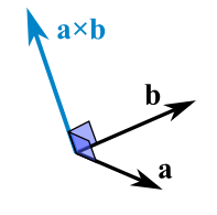
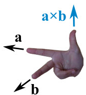
The cross product could point in the completely opposite direction and still be at right angles to the two other vectors, so we have the: Right Hand Rule.

CG

The magnitude (length) of the cross product equals the area of a parallelogram with vectors a and b for sides:

CG

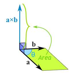
See how it changes for different angles:

CG

The cross product (blue) is:

  • zero in length when vectors a and b point in the same, or opposite, direction
  • reaches maximum length when vectors a and b are at right angles

And it can point one way or the other!

So how do we calculate it?

We can calculate the Cross Product this way:
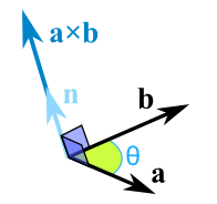
CG

1
a × b = |a|*|b|*sin(θ)*n
  • |a| is the magnitude (length) of vector a
  • |b| is the magnitude (length) of vector b
  • θ is the angle between a and b
  • n is the unit vector at right angles to both a and b

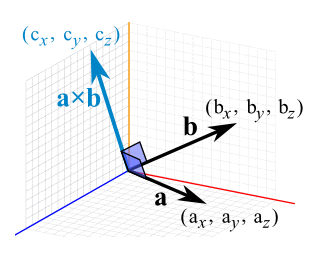
OR we can calculate it this way:
When a and b start at the origin point (0,0,0), the Cross Product will end at:

  • cx = aybz − azby
  • cy = azbx − axbz
  • cz = axby − aybx

CG


Next, there is a color attribute in our vertex called ‘SimpleVertex’. The color attribute is defined as a Colour type, which is also a self-defined type like ‘Vector4’. The color attribute stores a position’s color information, so that we can achieve lighting based on it. The inside of the ‘Colour’ type can also be regarded as a C++ struct, its structure is shown as below:

1
2
3
4
5
6
7
struct Colour 
{
float Red;
float Green;
float Blue;
float Alpha; // (In my final project, alpha is not used.)
};

Its outlined structure is so simple that only contains three float members to represent three primary colors of the light, including a number to represent the alpha.

Also, in order to use it in the real project more conveniently, basic APIs should be added into the ‘Colour’ structure above, as well as some more color-related APIs. The final structure of the color will be like the one below:

1
2
3
4
5
6
7
8
9
10
11
12
13
14
15
16
17
18
19
20
21
22
23
24
25
26
27
28
29
30
31
32
33
34
35
36
37
38
39
40
41
42
43
44
45
46
47
48
49
50
51
52
53
54
55
56
57
58
59
60
61
62
63
64
65
66
67
68
69
70
71
72
73
74
75
76
77
78
79
80
81
82
83
84
85
86
87
88
89
struct Colour 
{
Colour() = default;
Colour(const float red, const float green, const float blue) :
r(red), g(green), b(blue){}
Colour(const Colour& right)
{
this->r = right.r;
this->g = right.g;
this->b = right.b;
}

bool operator ==(const Colour& right)
{
if (this->r - right.r <= EPSILON
&& this->g - right.g <= EPSILON
&& this->b - right.b <= EPSILON)
{
return true;
}
else {
return false;
}
}

Colour& operator =(const Colour& right)
{
if (this == &right)
{
return *this;
}
this->r = right.r;
this->g = right.g;
this->b = right.b;
return *this;
}
Colour ClampColor(Colour& color)
{
Clamp(color.r, 0.f, 1.f);
Clamp(color.g, 0.f, 1.f);
Clamp(color.b, 0.f, 1.f);
return color;
}
Colour operator /(const float right) {
Colour result;
result.r = this->r / right;
result.g = this->g / right;
result.b = this->b / right;
return result;
}
Colour operator *(const Colour& right) const
{
Colour result;
result.r = this->r * right.r;
result.g = this->g * right.g;
result.b = this->b * right.b;
return result;
}
Colour operator *(const float& right) const
{
Colour result;
result.r = this->r * right;
result.g = this->g * right;
result.b = this->b * right;
return result;
}
Colour operator +(const Colour& right)
{
Colour result;
result.r = this->r + right.r;
result.g = this->g + right.g;
result.b = this->b + right.b;
return result;
}
Colour operator -(const Colour& right)
{
Colour result;
result.r = this->r - right.r;
result.g = this->g - right.g;
result.b = this->b - right.b;
return result;
}
Colour& operator *=(const Colour& right)
{
return (*this) = (*this * right);
}

float r, g, b;
};

One important thing to mention in the code above is the comparison of the two float-typed numbers. In computer, a float-type number may well not be the exact number we saw on log, it may hide subtle bias behind its decimal point, especially those float-type numbers after having mathematical operations. Remember that 1.0 - 1.0 in computer may not be 0 at all. To avoid this, we have to use subtraction and epsilon when comparing 2 float-type(or double-type) numbers. For example, if you want to know whether two float-type numbers are equal, subtraction of these two numbers is the first step, then just compare the subtracted result with the epsilon---a pretty tiny number that we have previously defined before. If the result is smaller than the epsilon, it means that the two float-type numbers are equal, vice versa.


Besides the basic APIs and operators we have mentioned above when talking about the ‘Vector4’, here we can see a different API called ‘ClampColor(Colour& color)’. As the word’s own meaning goes, the Clamp is a way to clamp some number in or der to make it into the range previously set, let’s just call that range ‘valid range’. So it is a simple conduction just to avoid the number being outside the bounds of range. For example, if you only want to ensure the digits you get are within the range of x and y, mathematically written as [x, y], you can just take y — which is the roof of the range — if some number is bigger than y, vice versa. The code below shows how does the clamping works:

1
2
3
4
5
6
7
8
float Clamp(const float& param, const float& min, const float& max)
{
if (param <= min)
return min;
else if (param >= max)
return max;
return param;
}

An optimization is just shown below:

1
2
3
4
float Clamp(const float& param, const float& min, const float& max)
{
return ((param < min) ? min : ((param > max) ? max : param));
}

But why we clamp colors?

As a common sense that we can use 01 or 0255 to represent a color’s attribute(R, G, B, A). In this case, we use 0~1. So this demands each of the color lies within the range of [0, 1]. In calculating float-type-based colors, because of the complex algorithm we use, it is almost possible that we gain a number outside the range we want. So clamping is always necessary.


The third member in our vertex is ‘Texcoord’, which represents texture coordinate, and its structure is very simple that only has two float-typed member, one is ‘U’ and the other is ‘V’. Just see the struct below:

1
2
3
4
5
struct Texcoord 
{
float U;
float V;
};

Texture coordinates, also called UVs, are pairs of numbers stored in the vertices of a mesh.

These numbers are often used to stretch a 2D texture onto a 3D mesh, but they can be used for other things like coloring the mesh, controlling the flow across the surface , etc.

Game engines commonly use two texture coordinates, U and V, for mapping the width and height of a texture. A third axis W can also be used for depth if you are using a 3D volume texture, but usually this coordinate is removed for efficiency.

Texture coordinates are measured in a scale of 0.0 to 1.0, with 0.0 and 1.0 at opposite sides of the texture. When a model has a UV distance greater than 1 (for example, UV goes from -1 to 2) then the texture will tile across the model.

These numbers are usually hidden from the artist, replaced by helpful visual representations of how the textures are projected. Planes, cylinders and spheres help the artist align the textures in a visual way, but it helps to know that games only see the UV numbers that these shapes create.

Texture coordinates define how an image (or portion of an image) gets mapped to a geometry. A texture coordinate is associated with each vertex on the geometry, and it indicates what point within the texture image should be mapped to that vertex.
Each texture coordinate is, at a minimum, a (u,v) pair, which is the horizontal and vertical location in texture space, respectively. The values are typically in the range of [0,1]. The (0,0) origin is at the lower left of the texture.
For (u,v) values outside the range of [0,1], the Texture Wrap Style property describes how this is handled.
Texture coordinates may also have optional values “w” and “q”. This is often represented as (u,v,w,q). These coordinates are both optional, so you may have, for example, (u,v,w) or (u,v,q).
The ‘w’ is used for more complex texture mapping in 3D space and is seen relatively infrequently in most workflows. This mapping in 3D may be in relation to 3D textures or 2D texture variations in 3D such as shadows. It can also be used with 2D textures that are intended to represent complex irregular surfaces in 3D.
The ‘w’ is used when rendering, in conjunction with the texture’s transformation values such as rotation, shearing, scaling, and offset. w is an extra value against which to multiply the texture transformation values, and may be used when you want to take perspective into account (such as in shadow mapping). It works the same as when you transform a location in object-space to 3D (solid) screen-space via a world-view-projection matrix. By multiplying the uvw with projection transformation values, you end up with two coordinates (often called s and t) which are then mapped onto a 2D texture.
The ‘q’ is used to scale texture coordinates when employing techniques such as projective interpolation. For most use cases, if a system can only handle (u,v) texture coordinates and is instead offered (u,v,q) values, a location of (u/q,v/q) may be used.


As we have took so much time on introducing the basic elements called ‘vertex’, we are sure that we have appropriate data structures to store the basic information of a 3D model. Let’s go on to the next step: Reading the model into the memory, which means that we are going to use our vertex-typed container to store each of the vertex from a 3D model. In C++, its convenient that we can use ‘vector’ in STL as a list to store all of the information we read from the model. Using ‘vector<SimpleVertex>‘ to represent a list of ‘SimpleVertex’ that we have just constructed above. Then comes the reading of a 3D model file. In this case we use OBJ format as it’s file structure is easier understand and visible in file format rather than a binary format like other model files. Lets take a simple look at the content of an file with OBJ format:

1
2
3
4
5
6
7
8
9
10
11
12
13
14
15
16
17
18
19
20
21
22
23
24
25
26
27
28
29
30
31
32
33
34
# File Created: 25.02.2021 17:35:16
# object Teapot001

v 0.279771417379 0.523323953152 0.361592650414
v 0.256112784147 0.523323953152 0.481412023306
v 0.252184033394 0.539422273636 0.479740440845
... ... ... ## details ignored
v 0.207081869245 0.542744159698 0.262634694576
v 0.235997557640 0.523323953152 0.250331819057
# 529 vertices

vn -0.966742336750 -0.255752444267 -0.000000119668
vn -0.893014192581 -0.256344825029 -0.369882434607
vn -0.893437385559 0.255995273590 -0.369101703167
vn -0.966824233532 0.255442529917 -0.000000077787
... ... ... ## details ignored
vn 0.350497841835 0.925311684608 -0.144739553332
vn 0.485588967800 0.850653529167 -0.201474279165
# 530 vertex normals

vt 2.000000000000 2.000000000000 0.000000000000
vt 1.750000000000 2.000000000000 0.000000000000
... ... ... ## details ignored
vt 0.375000000000 0.999999880791 0.000000000000
# 323 texture coords

o Teapot001
g Teapot001
f 1/1/1 2/2/2 3/3/3
f 3/3/3 4/4/4 1/1/1
... ... ... ## details ignored
f 528/250/529 471/254/472 473/256/474
f 473/256/474 529/252/530 528/250/529
# 1024 faces

The content of the OBJ file above is a pretty simple once, with many details ignored but the whole structure is entirely considered. The ‘#’ can be regarded as comments, there is no headers or tails in any OBJ files. Beginning with the vertex data, the ‘v’ represents the geometric vertices, ‘vt’ means ‘texture vertices’, ‘vn’ is ‘vertex normals’, and in some of the OBJ files there is ‘vp’, which means the parameter space vertices. Then comes the groups, ‘o’ is for the name of the object, ‘g’ is for the name of the group. The ‘f’ is crucial for it means ‘face’, the vertex indexes are split by ‘/‘, and always remember that the structure is mainly controlled by geometric vertices and the faces. We just stop deepening into the content of the file format as the detailed introduction about the OBJ file can be found online if you’re interested. Besides, you can even use FBX in your project rather than this kind of simple OBJ files.

Next, just I’m gonna show you the way to read OBJ file into our vertex container, namely, the computer memory we have constructed before. You can see that I divides the OBJ model data into the types(‘v’, ‘vt’, ‘vn’, ‘f’) before reading into the container just in accordance with the content of the files mentioned above.

1
2
3
4
5
6
7
8
9
10
11
12
13
14
15
16
17
18
19
20
21
22
23
24
25
26
27
28
29
30
31
32
33
34
35
36
37
38
39
40
41
42
43
44
45
46
47
48
49
50
51
52
53
54
55
56
57
58
59
60
61
62
63
64
65
66
67
68
69
70
71
72
73
74
75
76
77
78
79
80
81
82
83
84
85
86
87
88
89
90
91
92
93
94
95
96
97
98
99
100
101
102

void ReadOBJFileIntoOBJModel(const std::string& path, ModelInfo* obj)
{
std::ifstream in;
in.open(path, std::ifstream::in);
if (in.fail()) return;
if (in)
{
int vertexIndex = 0;
int vertexCount = 0;

std::vector<Vector4> verts;
std::vector<Vector3> texs;
std::vector<Vector4> norms;
std::string line;
float maxVx = -FLT_MAX, maxVy = -FLT_MAX, maxVz = -FLT_MAX;
float minVx = FLT_MAX, minVy = FLT_MAX, minVz = FLT_MAX;
while (!in.eof()) {
std::getline(in, line);
std::istringstream iss(line.c_str());
char trash;
if (!line.compare(0, 2, "v ")) {
iss >> trash;
float x, y, z;
iss >> x;
iss >> y;
iss >> z;
Vector4 v(x, y, z, 1.f);
Vertex newVertex;
newVertex.pos = v;
obj->vertexVec.push_back(newVertex);
vertexCount++;
maxVx = std::fmaxf(maxVx, v.getX());
maxVy = std::fmaxf(maxVy, v.getY());
maxVz = std::fmaxf(maxVz, v.getZ());
minVx = std::fminf(minVx, v.getX());
minVy = std::fminf(minVy, v.getY());
minVz = std::fminf(minVz, v.getZ());
}
else if (!line.compare(0, 3, "vt ")) {
iss >> trash;
iss >> trash;
float u, v;
iss >> u;
iss >> v;
if (u > 1.0f) u -= std::floor(u);
if (v > 1.0f) v -= std::floor(v);
obj->vertexVec[vertexIndex].tex = { u, v };
obj->vertexVec[vertexIndex].rhw = 1.0f;
vertexIndex++;
if (vertexIndex == vertexCount)
{
vertexIndex = 0;
}
}
else if (!line.compare(0, 3, "vn ")) {
iss >> trash;
iss >> trash;
float x, y, z;
iss >> x;
iss >> y;
iss >> z;
obj->vertexVec[vertexIndex].normal = Vector4(x, y, z, 0.f);
vertexIndex++;
if (vertexIndex == vertexCount)
{
vertexIndex = 0;
}
}
else if (!line.compare(0, 2, "f ")) {
std::vector<int> v;
std::vector<int> t;
std::vector<int> n;
int vx, vy, vz;
int tx, ty, tz;
int nx, ny, nz;

iss >> trash;
iss >> vx >> trash >> tx >> trash >> nx >>
vy >> trash >> ty >> trash >> ny >>
vz >> trash >> tz >> trash >> nz;

VerticeIndex indexes;
if (MODEL_PATH == "assets/Tonny.obj") {
indexes = { vx , vy, vz };
}
else
{
indexes = { vz , vy, vx }; // some obj files's vertex order is different (For Back Culling Correctly)
}
obj->verteciesIndexVec.push_back(indexes);
}
}
Vector4 center = Vector4((maxVx + minVx) / 2, (maxVy + minVy) / 2, (maxVz + minVz) / 2, 1.0f);

in.close();
}
else
{
std::cout << "No such file or path named \'" << path << "\' !" << std::endl;
}
}

By now, we have prepared a model data well. As you can see that the application stage is conducted in CPU, the programmer has the full control on every step and operation happened in this stage. You can try to reduce the count of the triangle during this stage in order to render it fast in the next stage, but the cost is obvious that the detail may lose. The CPU will send the data(model data which combined with vertices, vertices which includes positions, normals and texture coordinates) we stored into the hardware for the stage.


2. Geometry Stage

The model data prepared and sent from the application stage will be used as the input content for geometry stage. The main tasks of the geometry stage is to tranfer the vertices, do the clippings, shad lights, make projections and conduct screen mappings.

First and foremost, in order to make the mathematical calculations more unified, I have to mention that I use radiant(0~Π→0~180°) while describing an Euler angle, and use 0~1 rather than 0~255 while describing a color value, and use ‘vector • matrix’(vector-on-the-right-side) rule. The matrix are in ‘row-first’ order. Left-hand coordinate is used while doing geometric transforms.

In this stage there is a very important process called ‘MVP Transformation’, which is actually the combination of the ‘Model Transform’(the process during which we transform the model into its own space to the world space), ‘View Transform’(the process during which we transform the model from the world space into the view space) and the ‘Projection Transform’(the process during which we make the projection to the models in view space and transform it into the projection space). Let’s take a look at the detailed process of the geometry stage step by step.

Firstly, we have to transfer the model from its own space into the world space, but what is a ‘world space’? The world space is actually a space that holds all of the models, formally: objects. It should be able to hold all the objects with universal rules. The rule is originated from the world coordinates, which means that the world coordinate itself is a universal rule to all of the objects that are being rendered in the world space. Once we have learnt the origin of the universal rules, we are able to describe it in math, and you will find that describing a coordinate is simple in mathematics. It is a common sense that the coordinates can be easily described via matrix. As we can use a unit vector to form the base of a vector space, every vector in the space can be expressed as the linear combination of unit vectors, we can use a unit matrix to form the base of a matrix space. This means that the world space coordinate should be a unit matrix, so as to hold all the other objects. Thus the world space is created. Generally, we regard a unit matrix as a world space matrix, a world space, a world coordinate. A unit matrix is shown below, which can represent the world matrix. We can use a 3x3 matrix to represent a 3D space, but we choose 4x4 matrix, why? Because the position of our vertex is constructed in 4 dimension, with ‘w’ which represents the homogeneous coordinate. And we know that the mathematical rule does not allow us make arithmetic operations between a 3x3 matrix and a vector4. Also, the homogeneous coordinate W is crucial in the next steps that we can not lose it, we have to store it so as to use it later. As we use 2 dimentional array to define a matrix, we have to be clear about the inner side of it. In computing, row-major order and column-major order are methods for storing multidimensional arrays in linear storage such as random access memory. The difference between the orders lies in which elements of an array are contiguous in memory. In row-major order, the consecutive elements of a row reside next to each other, whereas the same holds true for consecutive elements of a column in column-major order. While the terms allude to the rows and columns of a two-dimensional array, i.e. a matrix, the orders can be generalized to arrays of any dimension by noting that the terms row-major and column-major are equivalent to lexicographic and co-lexicographic orders, respectively. Data layout is critical for correctly passing arrays between programs written in different programming languages. It is also important for performance when traversing an array because modern CPUs process sequential data more efficiently than non-sequential data. This is primarily due to CPU caching which exploits spatial locality of reference. In addition, contiguous access makes it possible to use SIMD instructions that operate on vectors of data. In some media such as tape or NAND flash memory, accessing sequentially is orders of magnitude faster than non-sequential access. We cannot clearly see whether the world matrix shown below is in row-major order or in column-major order for it is a unit matrix and the transpose of a unit matrix is actually itself, but I have to mention that all the matrices defined in this book and used in the relevant final project is in row-major order.

1
2
3
4
5
6
WorldMatrix = {
{1, 0, 0, 0}
{0, 1, 0, 0}
{0, 0, 1, 0}
{0, 0, 0, 1}
};

Then we have to place our models into the world space. As we have stored the model in a vertex which contains the attribute of position in 4 dimentional vector type, we can just multiply each of the position vectors with the world space matrix, thus transforming the positions of the model from its own space into the world space.

1
(type:matrix4f)ModelInWorldSpace = (type:vector4)ModelVertices[n].position * (type:matrix4f)WorldMatrix

Notice that all of the interactions on the object/models come from user side is applied on the models/objects in world space. This means that the rotation transform, scale transform and translation transform are conducted directly after we placed the models/objects in the world space through world matrix. First we have to map the user interaction from screen to 3D space if needed, for example, it’s needed that we map the rotation angle from 2D screen into 3D virtual world space if we want the user interact directly through the 2D screen when changing the rotation of the models/objects. Just multiplying the world matrix with the transform matrices will make the objects/models transform in the way we want. But how to describe our transform for the objects/models? Here are the details of the rotation matrix, scale matrix and transformation matrix that we should bear in mind:

Rotate by X-axis

1
2
3
4
5
6
RotationXMatrix = {
{1, 0, 0, 0}
{0, cos(θ), sin(θ), 0}
{0, -sin(θ), cos(θ), 0}
{0, 0, 0, 1}
};

Rotate by Y-axis

1
2
3
4
5
6
RotationYMatrix = {
{cos(θ), 0, -sin(θ), 0}
{0, 1, 0, 0}
{sin(θ), 0, cos(θ), 0}
{0, 0, 0, 1}
};

Rotate by Z-axis

1
2
3
4
5
6
RotationZMatrix = {
{cos(θ), sin(θ), 0, 0}
{-sin(θ), cos(θ), 0, 0}
{sin(θ), 0, 1, 0}
{0, 0, 0, 1}
};

The way to build out these matrices in C++ goes like the codes below:

1
2
3
4
5
6
7
8
9
10
11
12
13
14
15
16
17
18
19
20
21
22
23
24
25
26
27
28
29
30
31
32
33
34
35
36
37
38
39
40
41
42
43
44
45
46
47
48
49
50
51
52
53
54
55
56
57
   Matrix4f Matrix4f::getRotateXMatrix(const float& thetaX)
{
Matrix4f rotateXMatrix;

float angle = RadToDegree(thetaX);

rotateXMatrix.matrix[0][0] = 1.0f;
rotateXMatrix.matrix[3][3] = 1.0f;

float cosine = (float)cos(angle);
float sine = (float)sin(angle);
rotateXMatrix.matrix[1][1] = cosine;
rotateXMatrix.matrix[2][2] = cosine;
rotateXMatrix.matrix[1][2] = sine;
rotateXMatrix.matrix[2][1] = -sine;

return rotateXMatrix;
}

Matrix4f Matrix4f::getRotateYMatrix(const float& thetaY)
{
Matrix4f rotateYMatrix;

float angle = RadToDegree(thetaY);

rotateYMatrix.matrix[1][1] = 1.0f;
rotateYMatrix.matrix[3][3] = 1.0f;

float cosine = (float)cos(angle);
float sine = (float)sin(angle);
rotateYMatrix.matrix[0][0] = cosine;
rotateYMatrix.matrix[2][2] = cosine;
rotateYMatrix.matrix[0][2] = -sine;
rotateYMatrix.matrix[2][0] = sine;

return rotateYMatrix;
}

Matrix4f Matrix4f::getRotateZMatrix(const float& thetaZ)
{
Matrix4f rotateZMatrix;

rotateZMatrix.matrix[2][2] = 1.0f;
rotateZMatrix.matrix[3][3] = 1.0f;

float angle = RadToDegree(thetaZ);

float cosine = (float)cos(angle);
float sine = (float)sin(angle);
rotateZMatrix.matrix[0][0] = cosine;
rotateZMatrix.matrix[1][1] = cosine;
rotateZMatrix.matrix[0][1] = sine;
rotateZMatrix.matrix[1][0] = -sine;

return rotateZMatrix;
}

But notice that the direct rotation via Euler angles on any objects/models will cause Gimbal Lock. Gimbal lock is the loss of one degree of freedom in a three-dimensional, three-gimbal mechanism that occurs when the axes of two of the three gimbals are driven into a parallel configuration, “locking” the system into rotation in a degenerate two-dimensional space.
The word lock is misleading: no gimbal is restrained. All three gimbals can still rotate freely about their respective axes of suspension. Nevertheless, because of the parallel orientation of two of the gimbals’ axes there is no gimbal available to accommodate rotation about one axis.

CG

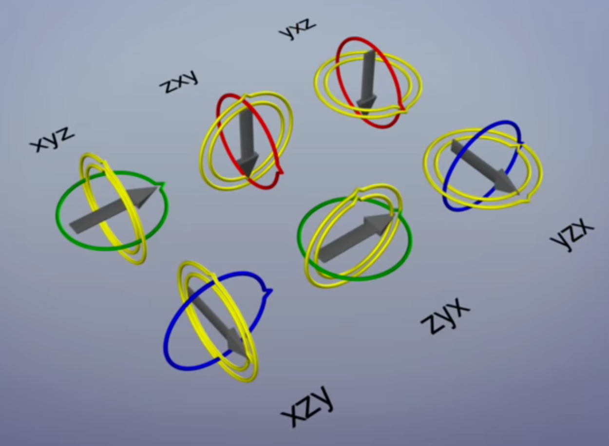
All together there are 6 parenting combinations to choose from. In each case gimbal lock occurs on the parent when the middle axis is rotated too far.

The cause of gimbal lock is the representation of orientation in calculations as three axial rotations based on Euler angles. A potential solution therefore is to represent the orientation in some other way. This could be as a rotation matrix, a quaternion , or a similar orientation representation that treats the orientation as a value rather than three separate and related values. Given such a representation, the user stores the orientation as a value. To quantify angular changes produced by a transformation, the orientation change is expressed as a delta angle/axis rotation. The resulting orientation must be re-normalized to prevent the accumulation of floating-point error in successive transformations. For matrices, re-normalizing the result requires converting the matrix into its nearest orthonormal representation. For quaternions, re-normalization requires performing quaternion normalization.

To avoid gimbal lock, we can use quaternion. Quaternion is a complex system in math.
In mathematics, the quaternion number system extends the complex numbers. Quaternions were first applied to mechanics in three-dimensional space. Hamilton defined a quaternion as the quotient of two directed lines in a three-dimensional space, or, equivalently, as the quotient of two vectors. Multiplication of quaternions is noncommunicative. Quaternions are used in pure mathematics, but also have practical uses in applied mathematics, particularly for calculations involving three-dimensional rotations, such as in three-dimensional computer graphics, computer vision, and crystallographic texture analysis. They can be used alongside other methods of rotation, such as Euler angles and rotation matrices, or as an alternative to them, depending on the application. It can avoid Gimbal Lock.

The detail of an angle’s quaternion is a matrix shown below:
Quaternion matrix to describe the rotation

1
2
3
4
5
6
7
8
9
10
StartPoint(x1, y1, z1, 1)
EndPoint(x1, y1, z1, 1)
EulerAngle<StartPoint, EndPoint> = θ
Quaternion
= (
(StartPoint ⊗ EndPoint).x,
(StartPoint ⊗ EndPoint).y,
(StartPoint ⊗ EndPoint).z,
(StartPoint • EndPoint), // ==> cos(θ / 2)
)

The Euler angle between start point and the end point: θ, can be inversely calculated out through a quaternion for test, and it is equal to 2*arccos(Quaternion.w) when being inverted.

Here is the detailed method to get quaternion in real code:

1
2
3
4
5
6
7
8
9
10
11
12
13
14
15
16
17
18
19
20
21
22
23
24
25
26
27
28
29
30
31
Vector4 GetQuaternion(const Vector2 & lastPointV2, const Vector2 & curPointV2)
{
Vector4 result;

Vector3 lastPointV3;
Vector3 curPointV3;
ArcBallTransform(lastPointV2, lastPointV3);
ArcBallTransform(curPointV2, curPointV3);

Vector3 perp;
perp = lastPointV3 ^ curPointV3;

if (perp.getLength() > EPSILON)
{
result.setX(perp.getX());
result.setY(perp.getY());
result.setZ(perp.getZ());
// w=cos(rotationAngle/2) ---> formula
result.setW(lastPointV3 * curPointV3);
}
else
{
result.setX(.0f);
result.setY(.0f);
result.setZ(.0f);
result.setW(.0f);
}

///std::cout << "rotated (in degree)" << RadToDegree(2 * acosf(result.getW())) << std::endl;
return result;
}

You can see that the function above includes a function called ArcBallTransform, which is a mathematical way to map the 2D point onto a 3D sphere, thus making it possible to describe the user's interaction from 2D screen to 3D virtual world space. The detail of the arc ball transform goes like the code shown below:

1
2
3
4
5
6
7
8
9
10
11
12
13
14
15
16
17
18
19
20
21
22
23
24
25
26
27
28
29
30
31
32
33
34
35
36
37
38
39
40
41
42
43
44
   float GetKFactorForArcBall(const float para)
{
// mouse point ranges from [0, window_width - 1]
return 1.f / ((para - 1.f) * 0.5f);
}

void ArcBallTransform(const Vector2& pointOnScreen, Vector3& pointOnSphere)
{
// convert width&height to [-1,1], left-hand coordinate
Vector2 tempVec2((pointOnScreen.getX() * GetKFactorForArcBall(WINDOW_WIDTH)) - 1.f, (pointOnScreen.getY() * GetKFactorForArcBall(WINDOW_HEIGHT)) - 1.f);
//Vector2 tempVec2((pointOnScreen.getX() * GetKFactorForArcBall(WINDOW_WIDTH)) - 1.f,1.f - (pointOnScreen.getY() * GetKFactorForArcBall(WINDOW_HEIGHT))); // left-hand coordinate
float length = pow(tempVec2.getX(), 2) + pow(tempVec2.getY(), 2);

// if it's outside the ball
if (length > 1.f)
{
// scale to sphere
float norm = -1.f / sqrtf(length);

pointOnSphere.setX(tempVec2.getX() * norm);
pointOnSphere.setY(tempVec2.getY() * norm);
pointOnSphere.setZ(0.f);
}
// if it's inside the ball
else
{
pointOnSphere.setX(tempVec2.getX());
pointOnSphere.setY(tempVec2.getY());
pointOnSphere.setZ(sqrtf(1.f - length));
}
}

float GetArcAngleCosineValue(const Vector3& position, const Vector3& startPosition, const Vector3& endPosition)
{
float r = position.getZ();
float pointDistance =
sqrtf(
pow((endPosition.getX() - startPosition.getX()), 2)
+ pow((endPosition.getY() - startPosition.getY()), 2)
+ pow((endPosition.getZ() - startPosition.getZ()), 2));
float consAngle = (pow(r, 2) + pow(r, 2) - pow(pointDistance, 2)) / (2 * r * r); // cosine formula
return consAngle;
}

Changing the location(Translating the objects/models) directly from the screen-side(eg: the user clicked to select an object and moved the mouse from one point on screen to the other just to make the selected object move as the mouse’s track) is also in the same way I have mentioned above, but is much easier than doing rotation via arc ball transform plus quaternion. Only the subtraction of the 2 points is needed without any complicated calculations. However, the selection of the object/model in virtual 3D world space from 2D screen is a little bit hard for most of the fresh-hands for it demands some more bounding-box related algorithms and knowledge basis to achieve this.

Now here is the details of the translation transform matrix, through which we are able to translate an object from one place to another in a 3D world space:

1
2
3
4
5
6
TranslationMatrix = {
{1, 0, 0, 0}
{0, 1, 0, 0}
{0, 0, 1, 0}
{x, y, z, 1}
};

And here is the way to get the translation matrix in C++:

1
2
3
4
5
6
7
8
9
10
11
12
13
14
15
Matrix4f Matrix4f::getTranslateMatrix(const float& x, const float& y, const float& z)
{
Matrix4f translationMatrix;

translationMatrix.matrix[0][0] = 1.0f;
translationMatrix.matrix[1][1] = 1.0f;
translationMatrix.matrix[2][2] = 1.0f;
translationMatrix.matrix[3][3] = 1.0f;

translationMatrix.matrix[3][0] = x;
translationMatrix.matrix[3][1] = y;
translationMatrix.matrix[3][2] = z;

return translationMatrix;
}

After the translation, we might need some ways to scale the models/objects in 3D world space so that the things can be in the size we expected. Here is the detail of the scale matrix:

1
2
3
4
5
6
ScaleMatrix = {
{x, 0, 0, 0}
{0, y, 0, 0}
{0, 0, z, 0}
{0, 0, 0, 1}
};

Here are 2 ways to get the scale matrix in C++:

1
2
3
4
5
6
7
8
9
10
11
12
13
14
15
16
17
18
19
20
21
22
23
Matrix4f Matrix4f::getScaleMatrix(const float& x, const float& y, const float& z)
{
Matrix4f scaleMatrix;

scaleMatrix.matrix[0][0] = x;
scaleMatrix.matrix[1][1] = y;
scaleMatrix.matrix[2][2] = z;
scaleMatrix.matrix[3][3] = 1.0f;

return scaleMatrix;
}

Matrix4f Matrix4f::getScaleMatrix(const Matrix4f & matrixToScale, const float scaleFactor)
{
Matrix4f result;

for (int i = 0; i < 4; i++) {
for (int j = 0; j < 4; j++)
result.matrix[i][j] = matrixToScale.matrix[i][j] * scaleFactor;
}

return result;
}

All the transforms in world space from either the user interaction or the preset automation is conducted through matrices. The vertices multiplies the world space matrix, translation matrix, scale matrix as well as rotation matrix, the order of multiplying with the scale matrix, translation matrix and rotation matrix can be various be they should always be on the right side of the multiplication when using the ‘vector • matrix’(vector-on-the-right-side) rule. Otherwise, the transpose of them is needed to carry out the transformations correctly.

The formula goes like this:

1
ModelInWorldSpaceAfterScaling = ModelInWorldSpace * ScaleMatrix
1
ModelInWorldSpaceAfterRotation = ModelInWorldSpace * RotationMatrix
1
ModelInWorldSpaceAfterTranslation = ModelInWorldSpace * TranslationMatrix
1
ModelInWorldSpaceAfterTransform = ModelInWorldSpace * ScaleMatrix * RotationMatrix * TranslationMatrix

The second step is to transform the model from the world space into the view space. In order to create a view space, we have to construct a camera first. The main functions of this camera is to shot the models in scene and send the rendering data onto screen so that we can see what’s happening in the virtual 3D world. You can either separate the camera out as a single class or just inject it into the one of the class you think injectable and appropriate.

Before constructing a camera, we should learn the main function that the camera has to do for us while rendering. To make it more specific, the camera can be regarded as our eyes in the virtual 3D world, and in this way you’re going to realize the first thing the camera have to solve: seeing the models. How to see those models in the scene? There should be some rules so that the view is in correct and non-distorted state. Here are some rules we have to consider:

  1. The up-axis of the camera [In order to view the models/objects correctly];
  2. The position we are viewing the models from [We have to keep a distance from the models we want to see so that we can see them];
  3. The target of the camera that is shooting [In oder to specify the shooting position];

These three aspects are crucial for a camera to shoot the models or objects in a 3D space correctly, so we are going to build up a way to describe the way a camera shoots the scene. In computer graphics, we still use a matrix to describe the way, but there are 2 types of rule that the one is in left-hand coordinate while the other is in right-hand coordinate. Just use the one that you will not change in the future. In this book I use the left hand coordinate system in building up my camera matrix, which is called “LookAtMatrix” formally in the project. Let’s just take a look at the details of the view matrix we are going to use:

1
2
3
4
5
6
7
8
9
10
11
12
13
14
15
16
17
18
19
20
21
22
23
24
25
26
27
28
29
30
31
32
33
34
35
36
37
38
Matrix4f getLookAtMatrixForLeftHandCoordinate(Vector3 * eyePos, const Vector3 * lookAt, const Vector3 * up, Vector3 & newCameraUpAxis)
{
Vector3 zAxis = *lookAt - *eyePos;
zAxis.Normalize();
Vector3 xAxis = *up ^ zAxis; // cross product
xAxis.Normalize();
Vector3 yAxis = zAxis ^ xAxis; // cross product
newCameraUpAxis = yAxis; // store the last up-axis for updating camera position

Matrix4f result;

/// when(major==raw) => do: below
result.matrix[0][0] = xAxis.getX();
result.matrix[0][1] = yAxis.getX();
result.matrix[0][2] = zAxis.getX();
result.matrix[0][3] = 0;
result.matrix[1][0] = xAxis.getY();
result.matrix[1][1] = yAxis.getY();
result.matrix[1][2] = zAxis.getY();
result.matrix[1][3] = 0;
result.matrix[2][0] = xAxis.getZ();
result.matrix[2][1] = yAxis.getZ();
result.matrix[2][2] = zAxis.getZ();
result.matrix[2][3] = 0;
result.matrix[3][0] = -(xAxis * (*eyePos));
result.matrix[3][1] = -(yAxis * (*eyePos));
result.matrix[3][2] = -(zAxis * (*eyePos));
result.matrix[3][3] = 1;

/*
Matrix-Structure(
xaxis.x, yaxis.x, zaxis.x, 0,
xaxis.y, yaxis.y, zaxis.y, 0,
xaxis.z, yaxis.z, zaxis.z, 0,
-xaxis.Dot(eyePos), -yaxis.Dot(eyePos), -zaxis.Dot(eyePos), 1
);*/
return result;
}

It’s just creating a virtual camera for shooting the virtual 3D world using matrix. Ones all the significant information is stored in the matrices, it will be so easy for us to apply them onto the models in the 3D world be rendered. The result of the matrix we gain via the function above is the origin of our view matrix. So we apply the matrix we gain by using the function above to an empty matrix to store our view matrix. Now you will realize that you can directly regard the view matrix as the ‘camera matrix’ or ‘eye matrix’, any transforms conducted onto the camera shall directly be conducted on the view matrix.

Now that we gained the view matrix singly by configuring the camera we are using in the virtual 3D world, we can transform the vertices from the world space into the view space just by updating the vertices in the world space through: multiplying the vertex positions already in the world space with the view matrix.

1
ModelInViewSpace = ModelInWorldSpace * ViewMatrix;

Till now, we have successfully transformed the models from the world space into the view space, next step after this is the transform of the model from the view space into the projection space. In order to make the transform, we have to gain projection matrix first.

There are 2 kinds of projections in our life, the one is orthographic while the other is perspective.

In the orthographic projection, the things we see will be shown in the shape based on its original geometric shape, non-distorted surfaces with all of the lines and points mathematically-ordered. For this reason, we use a cube to project the objects/models in the view space, all the shapes are projected mathematically through a cube.

In the perspective projection, the things we see will be shown in the shape based on its realistic shape we see in our real life. It seems ‘realistic’ just because of the fact that the human eyes see things in perspective view, the shapes of the objects in real life is distorted when it is being projected into our brains from our eyes: mastering the rule that “Everything looks small in the distance and big on the contrary”. For this reason, we use cone to project the objects/models in the view space rather than a cube, all the shapes are projected from a point, also, the furthest objects will disappear and become as a point after the projection.

Since we have noticed the main difference of 2 types of projection, the question lingers: What elements are needed when acquiring the projection matrix?

As we use a geometry to make the projection process(using a cube to make the orthographic projection while using a cone to make the perspective projection), the properties of the geometry selected shall be the attributes we have to consider when making the projection. We store the projection space in a 4x4 matrix as we did for the world space and view space before.

A cube has its width, height and length. When projecting, it’s enough for us to build out an orthographic projection matrix using these 3 attributes. We use its length to represent the distance from the nearest z-position(zNear) to the furthest z-position(zFar). Any objects/models outside this range will not be seen and should be clipped away so that they will not be rendered on screen. We usually set a small number, for example 0.2 as the nearest z-position while a bigger like 500 as the furthest z-position. Conus left can be 0 while the conus right should be the width of the cube, conus bottom can be 0 while the conus top should be the height of the cube. Here is the details of the orthographic matrix:

1
2
3
4
5
6
7
8
9
10
11
12
13
14
Matrix4f Matrix4f::getOrthographicMatrix(const float conusLeft, const float conusRight, const float conusBottom, const float conusTop, float zNear, float zFar)
{
Matrix4f orthographicMatrix;
/// make z range : [0,1], left hand coordinate
orthographicMatrix.matrix[0][0] = 2.f / (conusRight - conusLeft);
orthographicMatrix.matrix[1][1] = 2.f / (conusTop - conusBottom);
orthographicMatrix.matrix[2][2] = 1.f / (zFar - zNear); // in left hand coordinate
orthographicMatrix.matrix[3][0] = -(conusRight + conusLeft) / (conusRight - conusLeft);
orthographicMatrix.matrix[3][1] = -(conusTop + conusBottom) / (conusTop - conusBottom);
orthographicMatrix.matrix[3][2] = -zNear / (zFar - zNear);
orthographicMatrix.matrix[3][3] = 1.f;

return orthographicMatrix;
}

A cone, however, is different from a cube, and it has not width or height. Apart form using its length to represent the distance from the nearest z-position(zNear) to the furthest z-position(zFar), we use its angle on roof to represent the viewing field, which is formally called: field of view. And there is another element we have to consider when building the perspective matrix, that is: aspect ratio, which is the ratio of the rendering view’s(or the image’s) width to its height, and is expressed with 2 numbers separated by a colon, such as 16:9. Its simple to gain the aspect ratio once we configured the target rendering height and width. In the final project accompanied with this book, I used 720 as window width and 576 as window height, which means the aspect ratio is 720:576. By now, we have all the important information gained from a cone to build out a perspective projection matrix, which represents the perspective projection space itself. Let’s take a look at the details of the perspective matrix below:

1
2
3
4
5
6
7
8
9
10
11
12
13
14
15
16
Matrix4f Matrix4f::getPerspectiveMatrix(float fovYOZ, float aspectRatio, float zNear, float zFar)
{
fovYOZ = DegreeToRad(fovYOZ);

float focalLength = 1.f / tanf(fovYOZ / 2);

Matrix4f perspectiveMatrix;

perspectiveMatrix.matrix[0][0] = focalLength / aspectRatio;
perspectiveMatrix.matrix[1][1] = focalLength;
perspectiveMatrix.matrix[2][2] = zFar / (zFar - zNear); // in left hand coordinate
perspectiveMatrix.matrix[3][2] = -(zFar * zNear) / (zFar - zNear);
perspectiveMatrix.matrix[2][3] = 1.f; // in left hand coordinate

return perspectiveMatrix;
}

Then the way to transform the vertices from the view space into the projection space is as easy as what we have done when transforming the vertices form the world space into the view space: multiplying the model information matrix in view space with one of the projection matrix we calculated above. The formula goes like this:

1
ModelInProjectionSpace = ModelInViewSpace * ProjectionMatrix;

Notice that we should choose one type of projection at a time so that we can view in relevant projection mode, so the exact formula in a frame goes like this:
When using perspective mode

1
ModelInPerspectiveProjectionSpace = ModelInViewSpace * PerspectiveProjectionMatrix;

When using orthographic mode

1
ModelInOrthographicProjectionSpace = ModelInViewSpace * OrthographicProjectionMatrix;

Till now we have successfully processed the MVP transform, here is the recitation of the MVP transform in a nut shell:

(matrices are all with type:matrix4f)
(positions are all with type:vector4)

1
ModelInWorldSpace = ModelVertices[n].position * WorldMatrix;
1
ModelInViewSpace = ModelInWorldSpace * ViewMatrix;
1
ModelInProjectionSpace = ModelInViewSpace * ProjectionMatrix;

After we have transformed the vertices into the relevant projection space(perspective or orthographic), we have to make clippings. Clipping is a way to ignore the vertices that need not to be rendered in our visible area. In formula, when a vertex is inside the frustum, its position in X-axis and Y-axis will lay among the range of [-w, w] while its position in Z-axis will be in the range of [0, w]. So we can use this formula to check whether a vertex is inside the frustum. Here is the detail of the way to check whether a vertex is inside the CVV:

1
2
3
4
5
6
7
8
9
10
11
12
   bool IsOutsideCVV(const Vector4& v)
{
float x = v.getX();
float y = v.getY();
float z = v.getZ();
float w = v.getW();

if (x <= w && x >= -w && y <= w && y >= -w && z <= w && z >= 0)
return false;

return true;
}

A similar step with clippings is back culling, which is a way to ignore the back side of the model being rendered so that the rendering efficiency may be accelerated. When culling the backside of the model being rendered in virtual 3D world space, the important thing is to figure out its normal. The normal is decided upon the rule of drawing triangle: if you draw a triangle by connecting the vertices clockwise, the back side of the model is pointed to the inner side to the screen, vice versa. We can easily figure out the normal based on the Right-hand Screw Rule, but in programming, we have to know the way to express the Right-hand Screw Rule: we make subtractions twice to take all the three points into consideration as well as pretending to screw from one point to the other, then we calculate the cross product of the first point with the second point(or the second with the third, as is shown using ‘way 2’ below, but the points must be in continuity so as to pretend the screwing correctly). This normalized cross-product result best describes the normal of three points — the triangle. The back side of a primitive is easily figured out in this way. Here is the detail of CVV-Clipping and back-culling in my simple project:

1
2
3
4
5
6
7
8
9
10
11
12
13
14
15
16
17
18
19
20
21
22
23
24
25
26
27
28
29
30
31
32
33
34
35
36
37
38
39
40
41
42
43
44
45
46
47
48
49
50
51
52
53
54
55
56
57
58
59
60
61
62
63
64
65
66
67
68
69
70

Vector4 GetNormalVectorForBackCulling(const Vector4& p1, const Vector4& p2, const Vector4& p3)
{
Vector4 s1, s2, pn;
s1 = p3 - p2;
s2 = p2 - p1;
pn = s1 ^ s2; //way 1
//Vector4 s3; s3 = p1 - p3; pn = s2 ^ s3; //way 2
pn.Normalize();
return pn;
}


bool ShouldCullBack(const Vector4& vec)
{
// anti-clock wise culling
Vector4 v(0.f, 0.f, 1.f, 0.f);
if (v * vec > 0) return false;
return true;
}

void DrawTriangle(Vertex& v1, Vertex& v2, Vertex& v3, const Colour** texture)
{
Vector4 pos1AfterMVP, pos2AfterMVP, pos3AfterMVP;

Vector4 pos1TransformedToWorld, pos2TransformedToWorld, pos3TransformedToWorld;
m_transform->ModelToWorld(pos1TransformedToWorld, v1.pos);
m_transform->ModelToWorld(pos2TransformedToWorld, v2.pos);
m_transform->ModelToWorld(pos3TransformedToWorld, v3.pos);

v1.posInWorldSpace = pos1TransformedToWorld;
v2.posInWorldSpace = pos2TransformedToWorld;
v3.posInWorldSpace = pos3TransformedToWorld;

Vector4 pos1InView, pos2InView, pos3InView;
Vector4DotMatrix4f(pos1InView, pos1TransformedToWorld, m_transform->viewMatrix);
Vector4DotMatrix4f(pos2InView, pos2TransformedToWorld, m_transform->viewMatrix);
Vector4DotMatrix4f(pos3InView, pos3TransformedToWorld, m_transform->viewMatrix);

Vector4DotMatrix4f(pos1AfterMVP, pos1InView, m_transform->projectionMatrix);
Vector4DotMatrix4f(pos2AfterMVP, pos2InView, m_transform->projectionMatrix);
Vector4DotMatrix4f(pos3AfterMVP, pos3InView, m_transform->projectionMatrix);


Vector4 transformedVertNormal1, transformedVertNormal2, transformedVertNormal3;

// CVV Clip here
if (m_transform->IsOutsideCVV(pos1AfterMVP)
&& m_transform->IsOutsideCVV(pos2AfterMVP)
&& m_transform->IsOutsideCVV(pos3AfterMVP)) return; //The clipping happens here! Just stop here to prevent points from next steps.

m_transform->ModelToWorld(transformedVertNormal1, v1.normal);
m_transform->ModelToWorld(transformedVertNormal2, v2.normal);
m_transform->ModelToWorld(transformedVertNormal3, v3.normal);

Vector4 homogenizedVertPos1, homogenizedVertPos2, homogenizedVertPos3;
/// Set projection transform ---> To NDC
m_transform->Homogenize(homogenizedVertPos1, pos1AfterMVP);
m_transform->Homogenize(homogenizedVertPos2, pos2AfterMVP);
m_transform->Homogenize(homogenizedVertPos3, pos3AfterMVP);


Vector4 pn = GetNormalVectorForBackCulling(homogenizedVertPos1, homogenizedVertPos2, homogenizedVertPos3);
if (m_transform->ShouldCullBack(pn)) return; //The culling happens here! Just stop here to prevent the points from rasterization stage.


ScanLineDraw();
}


You can see that the points are just prevented from being sent to the rasterization stage when we are culling the back. The points are prevented from going to the next steps when clipping also.

There is a step not mentioned above that we may do before making the projection(inside the MVP, before ‘P’): shading lights. Shading lights is an operation conducted on textures of the models. When shading the light, lots of algorithms is used. In the final project asides this book, I showed the way of computing light and shading the light in Lambert mode. Main formula of Lambert Lighting is :

1
I = Ia * Ka + Ip * Kd * (N·L)
1
I = Ia * Ka + Ip * Kd * cosTheta;

The details of lighting are shown below:

1
2
3
4
5
6
7
8
9
10
11
12
13
14
15
16
17
18
19
20
21
22
23
24
25
26
27
28
29
30
31
32
33
34
35
36
37
38
39
40
41
42
43
44
45
46
47
48
49
50
51
52
53
54
55
56
57
58
59
60
61
62
63
64
65
66
67
68
69
70
71
72
73
74
75
76
77
78
79
struct Light
{
Vector3 direction;
Colour color;

Light(const Vector3& direction, const Colour& color) :direction(direction), color(color) {}
Light(const Colour& color) : color(color) {}
};

class DirectionalLight : public Light {
public:
// important to know that the initializer should be initiated from parent
DirectionalLight(const Colour& c, const Vector3& position, const Vector3& target, float intensity)
:Light(c), position(position), targetPosition(target), intensity(intensity) {}
DirectionalLight(const Colour& c, const Vector3& direction, float intensity)
:Light(Vector3::Normalize(direction), c), intensity(Clamp(intensity, 0.f, 1.f)) {}
~DirectionalLight() {}


// Global directional light using Lambert Shading
// I = Ia * Ka + Ip * Kd * (N·L)
// Ia * Ka --> ambient light
// back side will be totally black in the case of removing the ambient light
static void LambertLightOn(Colour& ambientColour, DirectionalLight* light, Vector3& normalInWorldSpace, Colour& vertexColor)
{
//float I, Ia, Ip, Kd, cosTheta;
float Ia, Ip, Kd, cosTheta;
Ia = 0.2f; //ambient light intensity
Ip = light->intensity; //directional light intensity
Kd = 1.f; //coefficients of directional light
light->direction.Normalize();
normalInWorldSpace.Normalize(); // must be normalized!!!
cosTheta = light->direction * normalInWorldSpace; // incident angel
cosTheta > 1.f ? (cosTheta = 1.f) : (cosTheta < 0.f ? cosTheta = 0.f : cosTheta = cosTheta);
////Formula: I = Ia * Ka + Ip * Kd * cosTheta;
Colour result = ambientColour * (Ia * Kd) + light->color * (Ip * Kd * cosTheta);
// clamp the colors' rgb value into valid range in case of bounding outside
if (result.r > 1.f || result.g > 1.f || result.b > 1.f)
result.r = result.g = result.b = 1.f;
else if (result.r < 0.f || result.g < 0.f || result.b < 0.f)
result.r = result.g = result.b = 0.f;
vertexColor = result;
}


void ComputeLighting(const DirectionalLight& light, const Vector3& P, const Vector3& N,
const Vector3& eyePosition, const float shininess,
Colour& diffuseResult, Colour& specularResult, const float attenuate)
{
// calculate diffuse
Vector3 L = (light.position - P);
L.Normalize();
float diffuseLight = max(N * L, 0); // always get the bigger value to ignore the error case such as shading from the back side
diffuseResult = light.color * diffuseLight * attenuate;

// calculate reflection
Vector3 V = eyePosition - P;
V.Normalize();
Vector3 H = L + V;
H.Normalize();
float specularLight = pow(max((N*H), 0), shininess);
if (diffuseLight <= 0) specularLight = 0;
specularResult = light.color * specularLight * attenuate;
}


private:
Vector3 targetPosition;
Vector3 position;
float intensity;

// calculate the normal vector of the light in world space coordinate
inline Vector3 DirectionInWorldSpace() {
Vector3 direction;
direction = position - targetPosition;
direction.Normalize();
return direction;
};
};

After the MVP transform and clippings, we know that the models state does not change at all, they are still in 3D state, but we have to see it on a 2D screen, so the screen mapping comes to help us transform the 3D vertices into the 2D screen. Screen mapping is a technic that maps the 3D vertices to the 2D screen. As is the codes shown above in function ‘DrawTriangle’, we simply call it Homogenize: the way to transform the vertices from the projection space into the screen space. Here is the detail of homogenizing a vertex:

1
2
3
4
5
6
7
8
9
10
11
   void Homogenize(Vector4& result, const Vector4& posInProjectionSpace)
{
if (posInProjectionSpace.W == 0) {
return Vector4();
}
float rhw = 1 / posInProjectionSpace.W;
result.X = (1 + posInProjectionSpace.X * rhw) * canvasWidth * 0.5; // screen coordinate
result.Y = (1 - posInProjectionSpace.Y * rhw) * canvasHeight * 0.5; //screen coordinate ---> top down
result.Z = posInProjectionSpace.Z * rhw;
result.W = rhw;
}

After such a long process, with the pixels we have just gain, we are entering into the next stage: rasterization stage, where we conduct multiple operations on each pixel so that each of the frame — namely an image, formed of many pixels — rendered on screen is in ideal state.


3. Rasterization Stage

The vertices we gain in screen space during the geometry stage will be used for drawing the final image, formally: single frame, that we are able to see directly.

After the screen mapping, through which we transformed the vertices from projection space to the screen space, some of the processes is still needed to make out a single frame to be rendered, and these processes are conducted in rasterization stage. Actually, it is the rasterization stage that converts vector information (composed of shapes or primitives) into a raster image (composed of pixels) for the purpose of displaying real-time 3D graphics.

During rasterization, each primitive is converted into pixels, while interpolating per-vertex values across each primitive. Rasterization includes clipping vertices to the view frustum, performing a divide by z to provide perspective, mapping primitives to a 2D viewport, and determining how to invoke the pixel shader. While using a pixel shader is optional, the rasterizer stage always performs clipping, a perspective divide to transform the points into homogeneous space, and maps the vertices to the viewport.

The positions[type:Vector4(x,y,z,w)] in each vertices, coming into the rasterizer stage are assumed to be in homogeneous clip-space. In this coordinate space the X axis points right, Y points up and Z points away from camera.

You may disable rasterization by telling the pipeline there is no pixel shader, and disabling depth and stencil testing. While disabled, rasterization-related pipeline counters will not update. There is also a complete description of the rasterization rules. Rasterization rules define how vector data is mapped into raster data. The raster data is snapped to integer locations that are then culled and clipped (to draw the minimum number of pixels), and per-pixel attributes are interpolated (from per-vertex attributes) before being passed to a pixel shader. There are several types of rules, which depend on the type of primitive that is being mapped, as well as whether or not the data uses multi-sampling to reduce aliasing. More related topics is available online and in this book we are just talking about the simple steps to create the usable pixels for rendering.

The vertices are placed in screen space after being clipped in projection space, but not formally, they are still in projection space de facto. Because we only clipped away the vertices outside the projected area, there are still vertices inside the projected area but outside the screen area. Different from the back culling, the vertices outside the screen area/space, which is also called: the view frustum, need to be clipped away not only for the reason that they are useless for rendering, but the consideration of those vertices may explode our frame buffer. Frame buffer is a container that stores all of the pixels going to be rendered on screen. Its volume is screenHeight*screenWidth large, so by now you will realize the importance of clipping of the vertices outside the screen space.

The RHW is the reciprocal of the homogeneous (clip space) w coordinate of a vertex (e.g., 1/w).
Recall that we must expand our 3D vectors to 4D vectors in order to be able to multiply them with 4x4 matrices (which we do because 4x4 matrices allow us to completely encode both rotational, translational, and scaling terms). In doing so we often set (or assume) the expanded fourth (w) component is 1 for model vertices, and the nature of the transforms we use to bring model-space vertices into world or view space doesn’t include any terms that alter the w component.
However, the typical perspective projection transformation often takes the follow general form which, when multiplied with a general view-space vertex vector (x,y,z,1), gives you a vector like (Ax, By, Cz + E, zD) — note that the resulting vertex has a w component that is proportional to the original input’s z component. Also note that the space you’re in after multiplication by this matrix is called clip space, because the nature of the transform has distorted the viewing frustum into a cuboid, the edges of which are much easier to perform clipping against.
After clipping, the graphics pipeline divided by the w component to scale things based on distance to give you the perspective effect. This division cannot be encoded in a matrix transform.
Now, division by w is the same as multiplication by the reciprocal of w, and the reason that you are required to give the reciprocal of the clip space w coordinate is probably a throwback to the time when division was significantly slower than multiplication. When you use pre-transformed vertices, the transformation from model to world to view to clip space is skipped, but the rest of the pipeline (division by w, conversion to window coordinates, and rasterization, obviously) must still happen. Since the projection transform was skipped, there is no basis for the pipeline to determine the w coordinate to divide by, so it asks you for it.

There are some interesting uses for the value, but for the most part people use pre-transformed vertices when doing 2D rendering, and in that case its most useful to set the RHW value to 1, which effectively causes the divide to be a no-op.

The detail of initiating the RHW is shown below:

1
2
3
4
5
6
7
8
9
void VertexRHWInit(Vertex& v)
{
v.rhw = 1 / v.pos.W;
v.tex.u *= v.rhw;
v.tex.v *= v.rhw;
v.normal.X = v.normal.X * v.rhw;
v.normal.Y = v.normal.Y * v.rhw;
v.normal.Z = v.normal.Z * v.rhw;
}

There are lots of ways to draw triangles when we have pixels in hand. Each of the way has its pros and cons and we have to choose the correct one to use. BUt in the final project, I provided multiple choices for learning. For example, you can use Point-by-Point Comparison Method to draw a line, it has its costs on performance but also has it advantage on some tiny models which ought to be rendered precisely. And, we can easily put some effects on each of the vertices when drawing the points. Here is the detail of the ‘Point-by-Point Comparison Method’:

1
2
3
4
5
6
7
8
9
10
11
12
13
14
15
16
17
18
19
20
21
22
23
24
25
26
27
28
29
30
31
32
33
34
35
36
37
38
39
40
41
42
43
44
45
46
47
48
49
50
51
52
   void DrawPoint(const Vector4& p, const Colour& color, const Texcoord& tc, const Vector3& normal)
{
int y = (int)p.getY();
int x = (int)p.getX();

if (y < 0 || y >= m_height) return;
if (x < 0 || x >= m_width) return;

float& z = m_zbuffer[y * m_width + x];

if (z < p.getZ()) return;

unsigned int fcolor = 0;

int s = GetState(m_state);

if (s & STATE_DRAW_COLOR)
{
fcolor = GetHEXColor(color);
}
else
{
Colour textureColor;
if (s & STATE_DRAW_TEX) {

if (m_interp == INTERP_NONE) {
int tx = (int)roundf((tc.u * (textureWidth - 1)));
int ty = (int)roundf((tc.v * (textureHeight - 1)));
textureColor = pixelColorData[ty][tx];
}
else
{
textureColor = BilinearInterp(pixelColorData, textureWidth, textureHeight, tc.u, tc.v);
}
}

// default ambient light
Colour ambient(0.f, 1.f, 1.f);
float ambientIntensity = AMBIENT_INTENSITY;

// influence of ambient
ambient.r *= ambientIntensity * textureColor.r;
ambient.g *= ambientIntensity * textureColor.g;
ambient.b *= ambientIntensity * textureColor.b;

//fcolor = (int(ambient.r * 255) << 16 | int(ambient.g * 255) << 8 | int(ambient.b * 255));
fcolor = GetHEXColor(Colour(ambient.r, ambient.g, ambient.b)); // simple functions of the code above
}

m_framebuffer[y][x] = fcolor;
z = p.getZ();
}

Here is the detail of the ‘Point-by-Point Comparison Method To Draw A Line’:

1
2
3
4
5
6
7
8
9
10
11
12
13
14
15
16
17
18
19
20
21
22
23
24
25
26
27
28
29
30
31
32
33
34
35
36
37
38
39
40
41
42
43
44
45
46
47
48
49
50
51
52
53
54
55
56
57
58
59
60
61
62
63

// Draw line via Point-by-Point Comparison Method
void DrawLine(const Vector4& p1, const Vector4& p2)
{
Colour color = GetColorFromHEX(m_foregroundColour);

Texcoord tex = { 0.f, 0.f };
Vector3 normal(0.f, 0.f, 0.f);

int x1, y1, x2, y2;
x1 = (int)p1.getX();
y1 = (int)p1.getY();
x2 = (int)p2.getX();
y2 = (int)p2.getY();

float y, x;
y = p1.getY();
x = p1.getX();

if (x1 == x2 && y1 == y2) {
DrawPoint(p1, color, tex, normal);
}
else if (x1 == x2) {
DrawPoint(p1, color, tex, normal);
int increment = (y1 < y2) ? 1 : -1;
while (1) {
y += increment;
if (increment == 1 && y >= y2) break;
if (increment == -1 && y <= y2) break;
Vector4 p(x, y, 0.f, 1.f);
DrawPoint(p, color, tex, normal);
}
DrawPoint(p2, color, tex, normal);
}
else if (y1 == y2) {
DrawPoint(p1, color, tex, normal);
int increment = (x1 < x2) ? 1 : -1;
while (1) {
x += increment;
if (increment == 1 && x >= x2) break;
if (increment == -1 && x <= x2) break;
Vector4 p(x, y, 0.f, 1.f);
DrawPoint(p, color, tex, normal);
}
DrawPoint(p2, color, tex, normal);
}
else {
DrawPoint(p1, color, tex, normal);
float t = (float)abs(x2 - x1) / abs(y2 - y1);
int xIncrement = (p1.getX() < p2.getX()) ? 1 : -1;
int yIncrement = (p1.getY() < p2.getY()) ? 1 : -1;
while (1) {
y += yIncrement;
if (yIncrement == 1 && y >= y2) break;
if (yIncrement == -1 && y <= y2) break;
x += t * xIncrement;
Vector4 p(x, y, 0.f, 1.f);
DrawPoint(p, color, tex, normal);
}
DrawPoint(p2, color, tex, normal);
}
}

You can also choose another ways to draw line. In the final project, I separated the conduction on the pixel in the way below:

1
2
3
4
5
6
7
8
9
10
11
12
13
14
15
16
17
18
19
20
21
22
23
24
25
26
27
28
29
30
   void DrawPixel(int x, int y, unsigned int hexColor)
{
if ((x < m_width) && ((y < m_height)) && ((x >= 0)) && ((y >= 0)))
{
m_framebuffer[y][x] = hexColor;
}
}

void DrawPixel(const Vector2 & point, unsigned int hexColor)
{
int x = (int)point.getX();
int y = (int)point.getY();
DrawPixel(x, y, hexColor);
}

void DrawPixel(int x, int y, const Colour & color)
{
if ((x < m_width) && ((y < m_height))
&& ((x >= 0)) && ((y >= 0)))
{
m_framebuffer[y][x] = GetHEXColor(color);
}
}

void DrawPixel(const Vector2 & point, const Colour & color)
{
int x = (int)point.getX();
int y = (int)point.getY();
DrawPixel(x, y, color);
}

Besides this way, you can use Bresenhem Way to draw the line, here are the details:

1
2
3
4
5
6
7
8
9
10
11
12
13
14
15
16
17
18
19
20
21
22
23
24
25
26
27
28
29
30
31
32
33
34
35
36
37
38
39
40
41
42
43
44
45
46
   void DrawBresenhemLine(const Vector4 & startPoint, const Vector4 & endPoint)
{
if (startPoint == endPoint) return;

int x0 = (int)startPoint.getX();
int y0 = (int)startPoint.getY();
int x1 = (int)endPoint.getX();
int y1 = (int)endPoint.getY();

bool steep = false;
if (std::abs(x0 - x1) < std::abs(y0 - y1))
{
std::swap(x0, y0);
std::swap(x1, y1);
steep = true;
}
if (x0 > x1)
{
std::swap(x0, x1);
std::swap(y0, y1);
}
int dx = x1 - x0;
int dy = y1 - y0;
int derror2 = std::abs(dy) * 2;
int error2 = 0;
int y = y0;
for (int x = x0; x <= x1; ++x) {
if (steep) {
Colour co(1.f, 1.f, 1.f);
//DrawPixel(y, x, GetColorIntensity(co)); // way 1
Vector4 p((float)y, (float)x, 0.f, 0.f);
DrawPoint(p, co); // way 2
}
else {
Colour co(1.f, 1.f, 1.f);
//DrawPixel(x, y, GetColorIntensity(co)); // way 1
Vector4 p((float)x, (float)y, 0.f, 0.f);
DrawPoint(p, co); // way 2
}
error2 += derror2;
if (error2 > dx) {
y += (y1 > y0 ? 1 : -1);
error2 -= dx * 2;
}
}
}

The way to draw line in Bresenhem way shown above can even be optimized to the codes below:

1
2
3
4
5
6
7
8
9
10
11
12
13
14
15
16
17
18
19
20
21
22
23
24
25
26
27
28
29
30
31
32
33
34
35
36
37
38
39
40
41
42
43
44
45
46
47
48
49
50
51
52
53
54
55
56
57
58
59
60
61
62
63
64
65
66
67
68
69
70
71
72
73
74
75
76
77
78
79
80
81
82
83
84
85
86
87
88
89
90
91
92
93
94
95
96
97
98
99
100
101
102
103
104
105
106
107
108
109
110
111
112
113

void DrawBresenhemLineInUnoptimizedWay(const Vector4 & startPoint, const Vector4 & endPoint)
{
if (startPoint == endPoint) return;

float x1 = startPoint.getX();
float y1 = startPoint.getY();
float x2 = endPoint.getX();
float y2 = endPoint.getY();

float xTemp, yTemp;


/*1:Draw the line segment with no slope.*/

if (x1 == x2)
{
// avoid oversteping the boundary of visual plane
if (x1 > m_width || x1 < 0) return;

if (y1 > y2)
{
yTemp = y1;
y1 = y2;
y2 = yTemp;
}
for (float y = y1; y < y2&&y < m_height&& y >= 0; ++y)
{
DrawPixel(Vector2(x1, y), Colour(1.f, 1.f, 1.f));
}
return;
}


/*2:Draw the line segment with no slope.*/

// stipulate X1<X2, otherwise, swap them
if (x1 > x2)
{
xTemp = x1;
x1 = x2;
x2 = xTemp;

yTemp = y1;
y1 = y2;
y2 = yTemp;
}

float k = (y2 - y1) / (x2 - x1);

// 1:as the gradient factor is less than 1 or bigger than 0
if (k >= 0.0f&&k <= 1.f)
{
// draw pixel crosswise from x1 to x2 with attention of limiting inside window width
for (float x = x1, y = y1; x <= x2 && x >= 0 && x < m_width; ++x)
{
float dis = (x - x1) * k + y1 - y;
if (dis >= 0.5)
{
++y;
}
DrawPixel(Vector2(x, y), Colour(1.f, 1.f, 1.f));
}
}

// 2:as the gradient factor is less than 0 or bigger than -1
else if (k < 0.0f&&k >= -1.f)
{
for (float x = x1, y = y1; x <= x2 && x >= 0 && x < m_width; ++x)
{
float dis = (x - x1)*k + y1 - y;
if (dis < -0.5)
{
--y;
}
DrawPixel(Vector2(x, y), Colour(1.f, 1.f, 1.f));
}
}

// 3:as the gradient factor is bigger than -1
else if (k > 1.f)
{
float k1 = 1.f / k;
for (float y = y1, x = x1; y <= y2 && y >= 0 && y < m_height; ++y)
{
float dis = (y - y1)*k1 + x1 - x;
if (dis >= 0.5)
{
++x;
}

DrawPixel(Vector2(x, y), Colour(1.f, 1.f, 1.f));
}
}

// 4:as the gradient factor is less than -1
else if (k < -1.f)
{
float k1 = 1.f / k;
for (float y = y2, x = x2; y <= y1 && y < m_height && y >= 0; ++y)
{
float dis = (y - y2)*k1 + x2 - x;
if (dis <= -0.5)
{
--x;
}

DrawPixel(Vector2(x, y), Colour(1.f, 1.f, 1.f));
}
}
}

Once we are able to draw lines, we are able to draw triangles, too. By calling the method of drawing lines three times can we build out a triangle we want:

1
2
3
4
   //           startPoint,            endPoint
DrawLine(homogenizedVertPos1, homogenizedVertPos2);
DrawLine(homogenizedVertPos1, homogenizedVertPos3);
DrawLine(homogenizedVertPos2, homogenizedVertPos3);

Apart from this, we can use Scan-line Way to rasterize triangles on screen, which is the core of our rendering. The detail of the scan-line way is shown below:

1
2
3
4
5
6
7
8
9
10
11
12
13
14
15
16
17
18
19
20
21
22
23
24
25
26
27
28
29
30
31
32
33
34
35
36
37
38
39
40
41
42
43
44
45
46
47
48
49
50
51
52
53
54
55
56
57
58
59
60
61
62
63
64
65
66
67
68
69
70
71
72
73
void ScanlineFill(const Vertex & leftPoint, const  Vertex & rightPoint, const int yIndex, const Colour** texture)
{
float lineWidth = rightPoint.pos.getX() - leftPoint.pos.getX();
float step = 1.f;
if (lineWidth > 0.f) step = 1.f / lineWidth;
else return;

for (float x = leftPoint.pos.getX(); x <= rightPoint.pos.getX(); x++)
{
int xIndex = (int)(x + 0.5f);
float lerpFactor = (x - leftPoint.pos.getX()) / lineWidth;
float zValue = Lerp(leftPoint.pos.getZ(), rightPoint.pos.getZ(), lerpFactor);
if (xIndex >= 0 && xIndex < m_width && zValue > 0.f && zValue < 1.f) // clip again
{
float rhwTemp = Lerp(leftPoint.rhw, rightPoint.rhw, lerpFactor);

float& zInBuffer = m_zbuffer[yIndex * m_width + xIndex];

if (zValue < zInBuffer)
{
// Perpective correction! ---> useless in orthographic mode
float w = 1.f / rhwTemp;

zInBuffer = zValue; // write into z-buffer

// uv interpolation to get the texture color (multiplies w to gain perspective correction of uv-texcture)
float u = Lerp(leftPoint.tex.u, rightPoint.tex.u, lerpFactor) * w * (textureWidth - 1);
float v = Lerp(leftPoint.tex.v, rightPoint.tex.v, lerpFactor) * w * (textureHeight - 1);

int uIndex = (int)(u + 0.5f); // maybe this is more effective than (int)roundf(fNum)
int vIndex = (int)(v + 0.5f);

Colour vertexColor(1.f, 1.f, 1.f);

if (uIndex <= textureWidth - 1 && uIndex >= 0
&& vIndex <= textureHeight - 1 && vIndex >= 0) {
if (mLightOn)
vertexColor = Lerp(leftPoint.color, rightPoint.color, lerpFactor);

Colour texColor;
if (m_interp == INTERP_BILINEAR) {
Colour** m_texture = (Colour**)texture;
texColor = BilinearInterp(m_texture, textureWidth, textureHeight, u, v);
}
else {
texColor = texture[uIndex][vIndex];
}

float xHere = Lerp(leftPoint.posInWorldSpace.getX(), rightPoint.posInWorldSpace.getX(), lerpFactor);
float yHere = Lerp(leftPoint.posInWorldSpace.getY(), rightPoint.posInWorldSpace.getY(), lerpFactor);
float zHere = Lerp(leftPoint.posInWorldSpace.getZ(), rightPoint.posInWorldSpace.getZ(), lerpFactor);
posInWorldSpace = Vector4(xHere, yHere, zHere, 1.f); // For showing shadow of the models on the floor

Vector4DotMatrix4f(lightScreenPosBeforsHomogenized, posInWorldSpace, lightSpaceMatrix);
m_transform->Homogenize(posInLightScreen, lightScreenPosBeforsHomogenized);

int hX = (int)(posInLightScreen.getX() + 0.5f);
int hY = (int)(posInLightScreen.getY() + 0.5f);

float bias = GetBiasDynamically(biasDelta, rightPoint.normal, leftPoint.normal, lerpFactor);

if (hX > 0 && hY > 0 && hX < m_width && hY < m_height) {
if (posInLightScreen.getZ() - bias > depthBufferFromLightPos[hY * m_width + hX])
texColor *= Colour(0.3f, 0.3f, 0.3f);
}

m_framebuffer[yIndex][xIndex] = GetHEXColor(vertexColor * texColor);
}
}
}
}
}

You can see that we conduct Bilinear Interpolcation in rasterization stage, its a way of avoiding the edges of the texture mapped on the models/pbjects. The details of ‘Bilinear Interpolcation’ is shown below:

1
2
3
4
5
6
7
8
9
10
11
12
13
14
15
16
17
18
19
20
21
22
23
24
25
26
27
28
29
30
31
32
33
34
35
36
37
38
39
40
41
42
43
44
45
46
47
48
49
50
51
52
53
Colour BilinearInterp(Colour** textureColorData, const int textureWidth, const int textureHeight, const float u, const float v)
{
//float y = u * textureHeight, x = v * textureWidth;
float y = v, x = u;

int x0 = (int)floorf(x);
int y0 = (int)floorf(y);
int x1 = x0 + 1, y1 = y0 + 1;

// border correction
if (x0 < 0) {
x0 = 0;
x1 = 1;
x = 0;
}
if (y0 < 0) {
y0 = 0;
y1 = 1;
y = 0;
}
if (x1 > textureWidth - 1) {
x1 = textureWidth - 1;
x0 = textureWidth - 2;
x = (float)textureWidth - 1;
}
if (y1 > textureHeight - 1) {
y1 = textureHeight - 1;
y0 = textureHeight - 2;
y = (float)textureHeight - 1;
}


float w00 = (float)((y1 - y) * (x1 - x));
float w01 = (float)((y1 - y) * (x - x0));
float w11 = (float)((y - y0) * (x - x0));
float w10 = (float)((y - y0) * (x1 - x));


Colour c00 = textureColorData[x0][y0];
Colour c01 = textureColorData[x1][y0];
Colour c10 = textureColorData[x0][y1];
Colour c11 = textureColorData[x1][y1];

Colour interpedResult00 = c00 * w00;
Colour interpedResult01 = c01 * w01;
Colour interpedResult10 = c10 * w10;
Colour interpedResult11 = c11 * w11;

Colour c = interpedResult00 + interpedResult01 + interpedResult10 + interpedResult11;

return c;
}


When rasterizing, notice that the lerping is also needed in screen space for acquiring a correct pixel position on screen. More details of Lerping and resterizing triangles are shown below:

1
2
3
4
5
6
7
8
9
10
11
12
13
14
15
16
17
18
19
20
21
22
23
24
25
26
27
28
29
30
31
32
33
34
35
36
37
38
39
40
41
42
43
44
45
46
47
48
49
50
51
52
53
54
55
56
57
58
59
60
61
62
63
64
65
66
67
68
69
70
71
72
73
74
75
76
77
78
79
80
81
82
83
84
85
86
87
88
89
90
91
92
93
94
95
96
97
98
99
100
101
102
103
104
105
106
107
108
109
110
111
112
113
114
115
116
117
118
119
120
121
122
123
124
125
126
127
128
129
130
131
132
133
134
135
136
137
138
139
140
141
142
143
144
145
146
147
148
149
150
151
152
153
154
155
156
157
158
159
160
161
162
163
164
165
166
167
168
169
170
171
172
173
174
175
176
177
178
179
180
181
182
183
184
185
186
187
188
189
190
191
192
193
194
195
196
197
198
199
200
201
202
203
204
205
206
207
208
209
210
211
212
213
214
215
216
217
218
219
220
221
222
223
224
225
226

float Lerp(const float a, const float b, const float t)
{
if (t <= 0.f) return a;
else if (t >= 1.f) return b;
else return (b - a) * t + a; // optimized
}


Vector4 Lerp(const Vector4 vecA, const Vector4 vecB, const float t)
{
Vector4 result(
Lerp(vecA.getX(), vecB.getX(), t),
Lerp(vecA.getY(), vecB.getY(), t),
Lerp(vecA.getZ(), vecB.getZ(), t),
Lerp(vecA.getW(), vecB.getW(), t)
);
return result;
}

Vertex Lerp(const Vertex vecA, const Vertex vecB, const float t)
{
Vertex result{
Lerp(vecA.pos, vecB.pos, t),
Lerp(vecA.color, vecB.color, t),
Lerp(vecA.tex.u, vecB.tex.u, t),
Lerp(vecA.tex.v, vecB.tex.v, t),
Lerp(vecA.normal, vecB.normal, t),
Lerp(vecA.rhw, vecB.rhw, t),
Lerp(vecA.posInWorldSpace, vecB.posInWorldSpace, t)
};
return result;
}

Colour Lerp(const Colour& a, const Colour& b, float t)
{
Colour result;
result.r = Lerp(a.r, b.r, t);
result.g = Lerp(a.g, b.g, t);
result.b = Lerp(a.b, b.b, t);
return result;
}

void LerpVertexInScreenSpace(Vertex & v, const Vertex & v1, const Vertex & v2, float t)
{
//optimized below ---> using the inline Lerp functions rather than the one from Math.h
v.rhw = Lerp(v1.rhw, v2.rhw, t);
v.tex.u = Lerp(v1.tex.u, v2.tex.u, t);
v.tex.v = Lerp(v1.tex.v, v2.tex.v, t);
v.color = Lerp(v1.color, v2.color, t);
v.pos = Lerp(v1.pos, v2.pos, t);
v.normal = Lerp(v1.normal, v2.normal, t); // comment this line to stay normal unchanged(in world space)
v.posInWorldSpace = Lerp(v1.posInWorldSpace, v2.posInWorldSpace, t);
}

void DrawTopTriangle(const Vertex & p1, const Vertex & p2, const Vertex & p3, const Colour** texture)
{
for (float y = p1.pos.getY(); y <= p3.pos.getY() && y >= 0 && y < m_height; y += 0.5f)
{
int yIndex = (int)roundf(y);
if (yIndex >= 0 && yIndex < m_height)
{
float xl = (y - p1.pos.getY()) * (p3.pos.getX() - p1.pos.getX()) / (p3.pos.getY() - p1.pos.getY()) + p1.pos.getX();
float x2 = (y - p2.pos.getY()) * (p3.pos.getX() - p2.pos.getX()) / (p3.pos.getY() - p2.pos.getY()) + p2.pos.getX();

float dy = y - p1.pos.getY();
float t = dy / (p3.pos.getY() - p1.pos.getY());

// get the right and left point via interpolation
Vertex new1;
new1.pos.setX(xl);
new1.pos.setY(y);
LerpVertexInScreenSpace(new1, p1, p3, t);

Vertex new2;
new2.pos.setX(x2);
new2.pos.setY(y);
LerpVertexInScreenSpace(new2, p2, p3, t);

if (new1.pos.getX() < new2.pos.getX())
{
ScanlineFill(new1, new2, yIndex, texture);
}
else
{
ScanlineFill(new2, new1, yIndex, texture);
}
}
}
}

void DrawBottomTriangle(const Vertex & p1, const Vertex & p2, const Vertex & p3, const Colour** texture)
{
for (float y = p1.pos.getY(); y <= p2.pos.getY() && y >= 0 && y < m_height; y += 0.5f)
{
int yIndex = (int)roundf(y);
if (yIndex >= 0 && yIndex < m_height)
{
float xl = (y - p1.pos.getY()) * (p2.pos.getX() - p1.pos.getX()) / (p2.pos.getY() - p1.pos.getY()) + p1.pos.getX();
float x2 = (y - p1.pos.getY()) * (p3.pos.getX() - p1.pos.getX()) / (p3.pos.getY() - p1.pos.getY()) + p1.pos.getX();

float dy = y - p1.pos.getY();
float t = dy / (p2.pos.getY() - p1.pos.getY());

// get the right and left point via interpolation
Vertex new1;
new1.pos.setX(xl);
new1.pos.setY(y);
LerpVertexInScreenSpace(new1, p1, p2, t);

Vertex new2;
new2.pos.setX(x2);
new2.pos.setY(y);
LerpVertexInScreenSpace(new2, p1, p3, t);

if (new1.pos.getX() < new2.pos.getX())
{
ScanlineFill(new1, new2, yIndex, texture);
}
else
{
ScanlineFill(new2, new1, yIndex, texture);
}
}
}
}

void TriangleRasterization(const Vertex & p1, const Vertex & p2, const Vertex & p3, const Colour** texture)
{
if (p1.pos.getY() == p2.pos.getY())
{
if (p1.pos.getY() < p3.pos.getY())
{// Flat top
DrawTopTriangle(p1, p2, p3, texture);
}
else
{// Flat bottom
DrawBottomTriangle(p3, p1, p2, texture);
}
}
else if (p1.pos.getY() == p3.pos.getY())
{
if (p1.pos.getY() < p2.pos.getY())
{// Flat top
DrawTopTriangle(p1, p3, p2, texture);
}
else
{// Flat bottom
DrawBottomTriangle(p2, p1, p3, texture);
}
}
else if (p2.pos.getY() == p3.pos.getY())
{
if (p2.pos.getY() < p1.pos.getY())
{// Flat top
DrawTopTriangle(p2, p3, p1, texture);
}
else
{// Flat bottom
DrawBottomTriangle(p1, p2, p3, texture);
}
}
else
{// Segment the triangle
Vertex top;

Vertex bottom;
Vertex middle;
if (p1.pos.getY() > p2.pos.getY() && p2.pos.getY() > p3.pos.getY())
{
top = p3;
middle = p2;
bottom = p1;
}
else if (p3.pos.getY() > p2.pos.getY() && p2.pos.getY() > p1.pos.getY())
{
top = p1;
middle = p2;
bottom = p3;
}
else if (p2.pos.getY() > p1.pos.getY() && p1.pos.getY() > p3.pos.getY())
{
top = p3;
middle = p1;
bottom = p2;
}
else if (p3.pos.getY() > p1.pos.getY() && p1.pos.getY() > p2.pos.getY())
{
top = p2;
middle = p1;
bottom = p3;
}
else if (p1.pos.getY() > p3.pos.getY() && p3.pos.getY() > p2.pos.getY())
{
top = p2;
middle = p3;
bottom = p1;
}
else if (p2.pos.getY() > p3.pos.getY() && p3.pos.getY() > p1.pos.getY())
{
top = p1;
middle = p3;
bottom = p2;
}
else
{
// 3 points colinear
return;
}

// get middle X by interpolation, get coeffiecient-t first
float middleX = (middle.pos.getY() - top.pos.getY()) * (bottom.pos.getX() - top.pos.getX()) / (bottom.pos.getY() - top.pos.getY()) + top.pos.getX();
float dy = middle.pos.getY() - top.pos.getY();
float t = dy / (bottom.pos.getY() - top.pos.getY());

// get the right and left point via interpolation
Vertex newMiddle;
newMiddle.pos.setX(middleX);
newMiddle.pos.setY(middle.pos.getY());
newMiddle.normal = middle.normal;
LerpVertexInScreenSpace(newMiddle, top, bottom, t);

DrawBottomTriangle(top, newMiddle, middle, texture);
DrawTopTriangle(newMiddle, middle, bottom, texture);
}
}

The final process of the rasterization stage is kind of like image processing, its main difference with the image processing is that the rasterization stage process vertices gain in geomotry stage, which means that the pixels are created and converted manually by the real vertices, while the image processing is to process an image from an pure pixel container: image itself. But there is no doubt that many conductions of image processing can be integrated from rasterization stage.


© Alexander Ezharjan

31st, March, 2022


Editor: Alexander Ezharjan

Using this method, the similarity index will be reduced enormously:

Experimental Use Only

  1. Write using Word;
  2. Export as PDF in Word;
  3. Open exported PDF;
  4. Export all the pages into multiple JPEG files;
  5. Create a new Word document and set its style of all borders to 0cm;
  6. Integrate all the JPEG files into the the Word document at once;
  7. Save the Word document created in step-6 as a PDF file;
  8. Combine the PDF file created in step-2 with the files created in step-7 to reduce the similarity rate of the paper.
  9. Eg. In my tested case, ‘final-opt-v1.pdf’ used only Page 7~11 as the image, the similarity index droped from 44% to 43%; while ‘final-opt-v2.pdf’ added Page 19~21 based on it, the similarity index dropped from 43% to 27%.


Note that the FILE SIZE MATTERS!
Reduce the file size as much as possible while keeping the resolution as high as possible!

Be kindly reminded that this is only an experiment for testing the qualification of using Turnitin as a formal way for submitting assignment RATHER THAN an approach for submitting the papers directly via the methods mentioned above.


Here are other formal ways to reduce similarity index better.

My Lectures & Micro-films & Videos

Editor: Alexander Ezharjan
  1. [PREFIX]/VpN2uhHLG_M
  2. [PREFIX]/jBY1V1uklxs
  3. [PREFIX]/MtCl0HI2JJE
  4. [PREFIX]/B59-yAfN-5c
  5. [PREFIX]/UfdyJO3H5mo
  6. [PREFIX]/uGPFPjTT2hE
  7. [PREFIX]/eh2bNNBGggU

I=utu
.
EF=//yo
PR=https:
X=be

Editor: Alexander Ezharjan
  1. 切割MP3,按时间准确切割
1
ffmpeg -i F:\源.mp3 -ss 00:20:00 -to 02:30:05 F:\目标文件.mp3
  1. MTS到MP4

说明:(-b 4m:码率是4M;-s 1280*720:这个是设定视频大小。这2个参数其实可以删掉)

1
ffmpeg -i F:\源.mts -b 4M -s 1280*720 F:\结果.mp4
  1. MP4到WMV
1
ffmpeg -i f:\视频.mp4 -b 4M f:\out.wmv
  1. MP4图像旋转

说明:主要参数: -vf “transpose=1” ,这里等于1是顺时针90度旋转;如果用手机录制的时候录反了,则执行2次这个操作就正过来了

1
ffmpeg -i f:\o.mp4 -vf "transpose=1" f:\o2.mp4
  1. MP4到MP4改尺寸
1
ffmpeg -i G:\源.mp4 -b 4M -s 640*340 g:\OUT.mp4
  1. MP4到MP4改尺寸加水印

说明:1: -vf “movie=logo.png [logo];[in][logo] overlay=10:20 [out]” 这里面的是加水印的参数,logo.png是我自己做的PNG水印,大小
300100,10:20是水印的位置,为了方便,就把logo.png拷贝到FFMPEg的bin目录下(必须放,加路径就失败),这样不用再加路径了 ;2: -b 2M 是用2M压缩率; 3: -s 640340 意思是图像分辨率改为640*340。

1
ffmpeg -i G:\源.mp4 -vf "movie=logo.png [logo];[in][logo] overlay=10:20 [out]" -b 2M -s 640*340 g:\OUT.mp4
  1. 快速剪切某段视频作为输出

说明:上面截取 H:\源.mpg 这个视频,从第0秒开始,到23分20秒,这样一段,保存到G:\out.mp4,注意参数必须是 -c copy ,这样执行起来特别快,也就不到半分钟就搞定。

1
ffmpeg -i H:\源.mpg -ss 0:0:0 -to 0:23:20 -c copy G:\OUT.MP4
  1. 该编码为H265,让MP4瘦身2/3,1G的MP4可以压缩到300M
1
ffmpeg -i 源.MP4 -vcodec libx265 -acodec copy F:\OUT.MP4
  1. WAV转换格式到amr
1
ffmpeg -i test.wav -acodec libamr_nb -ab 12.2k -ar 8000 -ac 1 wav2amr.amr
  1. 提取视频中的声音保存成一个mp3
1
ffmpeg -i 源.mp4 输出.mp3
  1. 要实现批量转换,可以直接用这个批处理文件
1
for %%i in (*.mkv) do ffmpeg.exe -i "%%i" -vcodec copy -acodec copy "%%~ni.mp4"
  1. 合并多个MP4为一个

方法一

1
ffmpeg -i INPUT1.MP4 -i INPUT2.MP4 -f FORMAT -acodec AUDIOCODEC -vcodec VIDEOCODEC -sameq OUTPUT.MP4

方法二

(1) 先创建一个文本文件 filelist.txt, 内容如下:(注意input1、2、3是你的文件的名字,都在该目录下)

1
2
3
file 'input1.mp4'
file 'input2.mp4'
file 'input3.mp4'

(2) 以上是这个文本文件的内容,保存后,在命令行执行

1
ffmpeg -f concat -i filelist.txt -c copy output.mp4
  1. 下载直播流
1
FFmpeg -i xxxxxxxxx.m3u8 -c copy out.mp4
  1. FFmpeg将MP4转换为M3U8

(1) 直接将MP4文件转成m3u8:

1
ffmpeg -i demo.mp4 -hls_time 10 -hls_list_size 0 -hls_segment_filename ene_%05d.ts ene.m3u8

(2) 如果已经是ts文件了,则只需要执行下方命令即可:

1
ffmpeg -i demo.ts -c copy -map 0 -f segment -segment_list playlist.m3u8 -segment_time 10 output%03d.ts

(3) 将大量分割成ts文件的视频片段全部转换成mp4视频片段 — 直接上批处理脚本:

1
2
for %%a in ("D:\VideoProjects\NewDemo\*.ts") do ffmpeg -i "%%a"   -vcodec copy -vcodec copy -f mp4 "D:\VideoProjects\NewDemo\NewMP4\%%~na.mp4"
pause

(4) 上面的 ffmpeg -i test.ts -acodec copy -vcodec copy -f mp4 test.mp4 是将ts文件转换为mp4文件的意思,再在其之上套了一层for循环,%%a就是每个文件,转换命令最末尾的%%~na是将文件保持原来的文件名的情况下进行输出,存放到指定文件夹的意思。

  1. mp4视频转flv
1
ffmpeg -i test.mp4 -acodec copy -vcodec copy -f flv test.flv 
  1. 将本地指定的demo.ts文件进行推流
1
ffmpeg -re  -i demo.ts  -c copy -f mpegts   udp://127.0.0.1:1997
  1. 强制把输出视频文件帧率改为 24 fps
1
ffmpeg -i input.avi -r 24 output.avi
  1. 对视频每个一秒截一个图并存在本地
1
ffmpeg -i out.mp4 -f image2 -vf fps=fps=1 out%d.png
  1. 每隔20秒截一个图
1
ffmpeg -i out.mp4 -f image2 -vf fps=fps=1/20 out%d.png
  1. 将视频转换为图片,一帧一图
1
ffmpeg -i out.mp4 out%4d.png


参考

官网

作者: 艾孜尔江·艾尔斯兰

49天效应旨在说明
全球西方的一些发达、最为先进的科学技术在国内普罗大众之间的广泛传播、达到国内一定程度上众所周知的地步所需要花费的时间约为49天

这种规律的掌握有利于对各类技术领域提前研究,甚至在商业领域进行推广和营销。

提出该效应的人是艾孜尔江·艾尔斯兰。


拿ChatGPT为例,首先报道此新闻的是西方技术相关媒体,而后在一周到两周的时间内,针对国内而言对此消息获悉最早的是一批以诸如微信公众号、抖音等为载体的小型科技类自媒体(非官方媒体),最后经过一系列传播,不断扩大,更多的非科技类媒体也便参与其中,使消息不断在更多人群中扩散,在49天的时间里形成了以大型媒体以及技术大厂为主体的新型传播样态。学界也涌入其中。

如下图显示的是ChatGPT的全球搜索趋势

49Effect

Editor: Alexander Ezharjan
  1. 使用 conda create -n carla python=3.7 命令安装虚拟环境出错,说网络连接异常,经久查询未果:
    在这里插入图片描述

  2. 在终端输入下面这些:

    1
    2
    3
    4
    conda config --add channels https://mirrors.tuna.tsinghua.edu.cn/anaconda/cloud/msys2/
    conda config --add channels https://mirrors.tuna.tsinghua.edu.cn/anaconda/cloud/conda-forge/
    conda config --add channels https://mirrors.tuna.tsinghua.edu.cn/anaconda/pkgs/free/
    conda config --set show_channel_urls yes
  3. 走进 C:/Users/USER_NAME/.condarc,删除内部的 -defaults 选项,保存退出;
    在这里插入图片描述

  4. 重新运行 conda create -n carla python=3.7 指令即可。


作者:艾孜尔江·艾尔斯兰

编者:艾孜尔江

摩西是统计(或称基于数据的)机器翻译(MT)的一个实现方法。这是该领域目前的主要方法,并被谷歌和微软等公司部署的在线翻译系统所采用。在统计机器翻译(SMT)中,翻译系统接受大量并行数据的训练(系统从中学习如何翻译小段),以及更大量的单语数据(系统从中学习目标语言应该怎么组织)。平行数据是两种不同语言的句子集合,它们是句子对齐的,因为一种语言的每个句子都与另一种语言中相应的翻译句子相匹配,它也被称为bitext。

摩西的训练过程接收平行数据,并使用单词和语言片段(即为短语)的同时出现来推断两种语言之间的对应关系。在基于短语的机器翻译中,这些对应关系仅在连续的单词序列之间,而在基于分层短语的机器翻译或基于语法的翻译中,更多关于句子的结构被添加到对应关系中。例如,一个分层的机器翻译系统可以知道德国hat
X gegessen 对应于英语中的ate
X,其中Xs能被任何德语-英语单词对所替换。在这些类型的系统中使用的额外结构可能或并不能从并行语料的语言分析得到。摩西还实现了基于短语的机器翻译的扩展,称为因式翻译,可以将额外的语言信息添加到基于短语的翻译系统中。

有关摩西翻译模型的更多信息,请参见摩西网站上关于基于短语的机器翻译系统,基于句法的翻译系统或基于因子的翻译系统。

无论您使用哪种类型的机器翻译模型,创建一个表现良好的翻译系统的关键都是大量优质数据(语料)。您可以使用许多免费的并行数据源来训练样本系统,比如:http://www.statmt.org/moses/?n=Moses.LinksToCorpora。但(通常)您使用的数据越接近您要翻译的语言类型,得到的结果就越好。这是使用像Moses这样的开源工具的优势之一,如果您拥有自己的数据,那么您可以根据需要定制自己的翻译系统,并且可能比通用翻译系统获得更好的性能。摩西用来训练翻译系统的过程中需要句子对齐的数据,但如果语料在文档级别对齐,则通常可以使用像hunalign这样的工具将其转换为句子对齐的数据。

Moses系统的组成部分

摩西系统的两个主要组成部分是训练管道和解码器。还有各种开源社区贡献的工具和实用程序。训练管道实际上是一组工具(主要用perl编写,有些用C
++编写),它们采用原始数据(并行语料和单语言)并将其转换为机器翻译模型。解码器是一个单独的C
++应用程序,给定一个训练有素的机器翻译模型和源句子,将源语句翻译成目标语言。

1.培训管道:

从培训数据生成翻译系统涉及各个阶段,这些阶段在培训文档和基线系统指南中有更详细的描述。这些作为管道被完成,并且可由摩西实验管理系统所控制,而Moses通常可以轻松地将不同类型的外部工具插入到培训管道中

数据在被用于训练之前需要做一些准备工作,标记文本并且将标记转换为标准案例。启发式用于删除看起来未对齐的句子对,并删除长句子。然后,并行的句子需要词对齐,通常使用
GIZA
++来完成,它实现了80年代在IBM开发的一组统计模型。这些词对齐被用于根据需要提取短语-短语翻译或分层规则,并且使用这些规则的语料库范围统计来估计概率。

翻译系统的一个重要部分是语言模型,一种使用目标语言中的单语言数据构建的统计模型,并由解码器用来尝试确保输出的流畅性。摩西依靠外部工具http://www.statmt.org/moses/?n=FactoredTraining.BuildingLanguageModel)进行语言模型构建。

创建机器翻译系统的最后一步是调优,其中不同的统计模型相互加权以产生最佳可能的翻译。摩西系统包含了最流行的调优算法的实现。

2.解码器

摩西解码器的工作是找到与给定源句子相对应的目标语言(根据翻译模型)的最高评分句子。解码器还可以输出候选的翻译的从好到坏的排序列表,并且还提供关于其如何做出决策的各种类型的信息(例如,它使用的短语-短语对应关系)。

解码器以模块化方式编写,并允许用户以各种方式改变解码过程,例如:

  • 输入:这可以是一个简单的句子,或者它可以用类似xml的元素的注释来指导翻译过程,或者它可以是更复杂的结构,如格子或混淆网络(例如,从语音识别的输出)

  • 翻译模型:这可以使用短语-短语规则或分层(也可能是句法)规则。它可以编译成二进制形式,以加快加载速度。它可以通过将额外的信息添加到翻译过程中来补充一些特性,例如阐明短语对的来源以控制他们的可靠性的特性。

  • 解码算法:解码问题是一个巨型的搜索问题,通常对于精确搜索来说太大了,而且Moses为这种搜索实现了几种不同的策略,例如基于堆栈,立方体修剪,图表解析等。

  • 语言模型:
    Moses支持几种不同的语言模型工具包(SRILM,KenLM,IRSTLM,RandLM),每种工具包都有自己的优点和缺点,添加一个新的LM工具包很简单。

Moses解码器还支持多线程解码(因为翻译具有很高的的并行性),并且如果您有权访问群集服务器,摩西提供启用多进程解码的脚本。

贡献工具

摩西有许多贡献工具,它们提供额外的功能和超越标准训练和解码管道的附加功能。这些包括:

  • Moses服务器:为解码器提供xml-rpc接口,需要安装xmlrpc-c。

  • Web翻译:一组脚本,使Moses可用于翻译网页

  • 分析工具:与参考文献相比,是一个可以对摩西输出进行分析和可视化的脚本。

还有用于评估翻译的工具,替代短语评分方法,用于加权短语表的技术的实现,用于减小短语表的规模的工具以及其他贡献工具。

一 安装相关依赖项:

在本教程中,我用来搭建Moses系统的服务器环境如下:

1
2
3
4
5
6
7
8
9
10
11
root\@VM-0-15-ubuntu:/home/ubuntu/mosesdecoder\# lsb_release -a

No LSB modules are available.

Distributor ID: Ubuntu

Description: Ubuntu 16.04.4 LTS

Release: 16.04

Codename: xenial

安装如下依赖:

1
2
sudo apt-get install build-essential git-core pkg-config automake libtool wget
zlib1g-dev python-dev libbz2-dev

从Github克隆Moses:

1
2
git clone <https://github.com/moses-smt/mosesdecoder.git>
cd mosesdecoder

运行以下命令安装最新的boost库,cmph (for
CompactPT,即C Minimal Perfect Hashing Library), irstlm (language model from
FBK, required to pass the regression tests),和 xmlrpc-c (for moses
server)。这些都会默认安装在你的当前工作目录的./opt路径。其中xmlrpc不是必须,但是如果将moses作为服务提供必须安装xmlrpc。

1
make -f contrib/Makefiles/install-dependencies.gmake

编译Moses:

1
2
3
4
5
6

./compile.sh [additional options]

\--prefix=/destination/path --install-scripts 安装到其他目录

\--with-mm 使用基于后缀数组的短语表

其中,MOSES
SERVER使你可以把MOSES解码器作为一个服务器进程来运行,发送给其的句子将通过XMLRPC来翻译。这意味着无论客户使用java,python,perl,php还是其它别的XMLRPC集合里有的语言来编码,MOSES进程都可以服务客户且分布式地服务客户。

XMLRPC是Userland
Software公司设计的一种格式:是一种使用HTTP协议传输XML格式文件来获取远程程序调用(Remote
Procedure
Call)的传输方式。远程程序调用简单地讲是指,一台机器通过网络调用另一台机器里的应用程序,同时将执行结果返回。一般一台机器作为服务器端,另一台作为客户端。服务器端需要轮询是否有客户端进行RPC请求。一个简单的例子。一台服务器提供查询当前时间的RPC服务。其他任何一台机器通过网络,使用客户端,都可以到该服务器查询当前的时间。

MLRPC是RPC机制的实现方式之一。采用XML语言作为服务器与客户端的数据交互格式,方便使用者阅读。XMLRPC可以用很多种语言实现,包括perl,phyon,c等。使用c与c++实现的库,就是XMLRPC-c。

Boost
1.48版本在编译Moses时会出现一个严重的bug。在有些Linux的分发版本中,比如Ubuntu
12.04,Boost库存在着这种版本的Boost库。在这种情况下,你必须要手动下载和编译Boost。

下载编译boost:

1
2
3
4
5
6
7
8
9
10
11
12

wget <https://dl.bintray.com/boostorg/release/1.64.0/source/boost_1_64_0.tar.gz>

tar zxvf boost_1_64_0.tar.gz

cd boost_1_64_0/

./bootstrap.sh

./b2 -j4 --prefix=\$PWD --libdir=\$PWD/lib64 --layout=system link=static install
\|\| echo FAILURE \#或者执行./b2安装在当前目录下

上述命令在文件夹lib64中创建文件夹,并不是在系统目录下。因此,你不必使用系统root权限来执行上述命令。然而,你需要告诉Moses如何找到boost。当boost被暗账好以后,你可以开始编译Moses,你需要用 –with-boost标记告诉Moses系统
boost安装在哪里。

下载安装cmph:

1
2
3
4
5
6
7
8
9
10
11
12
13
wget
http://www.mirrorservice.org/sites/download.sourceforge.net/pub/sourceforge/c/cm/cmph/cmph/cmph-2.0.tar.gz

tar zxvf cmph-2.0.tar.gz

cd cd cmph-2.0/

./configure --prefix= /usr/local/cmph
\#指定安装路径,这里我选择了/usr/local/cmph

Make

Make install

下载安装xmlrpc-c:

1
2
3
4
5
6
7
8
9
10
11
12
13
14

wget
https://launchpad.net/ubuntu/+archive/primary/+sourcefiles/xmlrpc-c/1.33.14-8build1/xmlrpc-c_1.33.14.orig.tar.gz

tar zxvf xmlrpc-c_1.33.14.orig.tar.gz

cd xmlrpc-c-1.33.14/

./configure --prefix= /usr/local/xmlrpc-c
\#指定安装路径,这里我选择了/usr/local/xmlrpc-c

Make

Make install

接下来,用bjam编译Moses:

1
2
3
./bjam --with-boost=/home/ubuntu/boost_1_64_0 --with-cmph=/usr/local/cmph
--with-xmlrpc-c=/usr/local/xmlrpc-c -j4

注意: –with-boost
后的路径为你自己安装时指定的路径,-j4 用于指定核心数。Moses可选的语言模型有IRSTLM,SRILM,KenLM.其中,KenLM已经默认包含在Moses工具包中。我们在这里使用Moses自带的语言模型工具KenLM,不再安装irstlm。

二 安装词对齐工具GIZA++

接下来,安装词对齐工具GIZA++:

1
2
3
4
5
6

git clone <https://github.com/moses-smt/giza-pp.git>

cd giza-pp

make

编译完成后,将生成三个二进制文件:

· giza-pp/GIZA++-v2/GIZA++

· giza-pp/GIZA++-v2/snt2cooc.out

· giza-pp/mkcls-v2/mkcls

记得在编译完之后将上面的三个文件拷到一个目录下,便于访问使用。如下面的命令所示,我是直接将其放在tools文件夹下的。

1
2
3
4
5
6
7
8

cd \~/mosesdecoder

mkdir tools

cp \~/giza-pp/GIZA++-v2/GIZA++ \~/giza-pp/GIZA++-v2/snt2cooc.out \\

\~/giza-pp/mkcls-v2/mkcls tools

编译创建好GIZA++后,有两种方式来使用它,一是在编译Moses时将GIZA++的地址作为选项参数。如果在编译Moses时没有指定GIZA++的地址,可以采用另外一个方法,那就是在训练语言模型时指明GIZA++三个可执行文件的路径,例如:

1
2
3
train-model.perl -external-bin-dir \$HOME/external-bin-dir

我在实际操作中,采用的是第二种方法,即在使用Moses时,给一个参数指明GIZA++路径。

三 语料准备

接下来,准备平行语料:

我的英汉平行语料来自联合国的网站提供的英汉平行语料,(https://conferences.unite.un.org/uncorpus/zh),大约1600万对。因我使用的服务器内存只有4G,所以将原文件分成30份,从中截取了约60万对用来做此次实验。

我们的英文语料为:un_en-zh23.en,汉语语料为:un_en-zh23.cn。

在准备训练翻译系统之前,我们需要对语料做如下的处理:

  1. tokenisation:这一步主要是在单词和单词之间或者单词和标点之间插入空白,以便于后续识别和其他操作。

对于英文语料,我们运行如下命令:

1
2
3
4
5
6

\~/mosesdecoder/scripts/tokenizer/tokenizer.perl -l en \\

\< \~/corpus/training/un_en-zh23.en \\

\> \~/corpus/un_en-zh23.tok.en

注:命令当中的~为Mosesdecoder的安装路径和语料所在的具体路径,下同

对于汉语语料。我们需要进行分词。在这里,我们使用清华大学自然语言处理与社会人文计算实验室研制推出的中文词法分析工具包(http://thulac.thunlp.org),具有中文分词和词性标注功能。具有能力强,准确率高,速度快的特点。具体使用方法请参照网页。在这里,我们使用Python版本来对中文语料进行分词,具体代码如下:

1
2
3
4
5
6
7
8
9
10

import thulac

thu1=thulac.thulac(user_dict="/home/ubuntu/corpus/un_en-zh_23/dict.txt",seg_only=True)

\#只进行分词,不进行词性标注

thu1.cut_f("/home/ubuntu/corpus/un_en-zh_23/un_en-zh23.cn",
"/home/ubuntu/corpus/un_en-zh_23/un_en-zh23.fc")
\#对un_en-zh23.cn文件内容进行分词,输出到un_en-zh23.fc

经过tokenisation,我们得到un_en-zh23.fc和un_en-zh23.tok.en两个文件。

  1. truecase:初始每句话的字和词组都被转换为没有格式的形式(例如统一为小写)。这有助于减少数据稀疏性问题。

Truecase首先需要训练,以便提取关于文本的一些统计信息

1
2
3
4
5
6
7
8
9
10
11
12
13

\~/mosesdecoder/scripts/recaser/train-truecaser.perl \\

\--model \~/corpus/truecase-model.en --corpus \\

\~/corpus/ un_en-zh23.tok.en

\~/mosesdecoder/scripts/recaser/train-truecaser.perl \\

\--model \~/corpus/truecase-model.cn --corpus \\

\~/corpus/ un_en-zh23.fc

经过此步,我们得到truecase-model.en和truecase-model.cn两个文件。

接下来,我们对tokenisation后的文件进行truecase:

1
2
3
4
5
6
7
8
9
10
11
12
13
14
15
16

\~/mosesdecoder/scripts/recaser/truecase.perl \\

\--model \~/corpus/truecase-model.en \\

\< \~/corpus/ un_en-zh23.tok.en \\

\> \~/corpus/ un_en-zh23.true.en

\~/mosesdecoder/scripts/recaser/truecase.perl \\

\--model \~/corpus/truecase-model.cn \\

\< \~/corpus/ un_en-zh23.fc \\

\> \~/corpus/un_en-zh23.true.cn

经过truecase,我们得到un_en-zh23.true.cn和un_en-zh23.true.en两个文件。

  1. cleaning:长句和空语句可引起训练过程中的问题,因此将其删除,同时删除明显不对齐的句子。
    1
    2
    3
    4
    5
    6
    7

    \~/mosesdecoder/scripts/training/clean-corpus-n.perl \\

    \~/corpus/ un_en-zh23.true cn en \\

    \~/corpus/ un_en-zh23.clean 1 80

    需要注意的是,这句命令会对truecase-model.en和truecase-model.cn两个文件同时进行清洗。经过clean,我们得到un_en-zh23.clean.en和un_en-zh23.clean.cn两个文件。

四 语言模型训练(Language Model Training)

语言模型的训练是为了保证能够产生流利的输出,所以要用目标语言来建立。本例的目标语言是汉语。在这里,我们使用Moses系统中内置的语言语言模型工具KenLM,当然,你也可以使用其他一些开源的语言模型工具,比如,IRSTLM,BerkeleyLM,SRILM等。接下来,我们建立一个合适的3元文语言模型。

建立文件夹lm,然后运行如下命令:

1
2
3
4
5
6
7

mkdir \~/lm

cd \~/lm

\~/mosesdecoder/bin/lmplz -o 3 \<\~/corpus/ un_en-zh23.true.cn \>
un_en-zh23.arpa.cn

你会看到建立语言模型的五个步骤:

1/5 Counting and sorting n-grams

2/5 Calculating and sorting adjusted counts

3/5 Calculating and sorting initial probabilities

4/5 Calculating and writing order- interpolated probabilities

5/5 Writing ARPA model =FE Name

此步我们生成un_en-zh23.arpa.cn
文件,接下来我们为了加载的更快一些,我们使用KenLm来对*.arpa.en文件二进制化。

1
2
3
4
5
6
7

\~/mosesdecoder/bin/build_binary \\

un_en-zh23.arpa.cn \\

un_en-zh23.blm.cn

当你看到绿色的SUCCESS字样时说明二进制化已经成功了。我们可以在这一步之后通过查询测试来判断训练的模型是否正确,运行如下的linux命令你会看到:

1
2
3
4
5
6
7
8
9
10
11
12
13
14
15
16
17
18
19
20
21
22
23

\$ echo "我 爱 我的 好姑娘" \\

\| \~/mosesdecoder/bin/query un_en-zh23.blm.cn

Loading statistics:

我=8872 2 -2.282969 爱=18074 1 -6.466906 我的=9416 1 -4.8714185

好姑娘=0 1 -6.4878592 \</s\>=2 1 -2.288369 Total: -22.397522 OOV: 1

Perplexity including OOVs: 30165.07396388977

Perplexity excluding OOVs: 9493.266676976866

OOVs: 1

Tokens: 5

Name:query VmPeak:151680 kB VmRSS:4088 kB RSSMax:136452 kB

user:0.008 sys:0 CPU:0.008 real:0.00995472

五 训练翻译模型(Training the Translation System)

接下来,我们进行到最主要的一步,训练翻译模型。在这一步,我们进行词对齐(用GIZA++),短语抽取,打分,创建词汇化重新排序表,并且创建属于我们自己的摩西配置文件(moses.ini)。我们运行如下的命令:

1
2
3
4
5
6
7
8
9
10
11
12
13
14
15

mkdir \~/working

cd \~/working

nohup nice \~/mosesdecoder/scripts/training/train-model.perl -root-dir train \\

\-corpus \~/corpus/ un_en-zh23.clean \\

\-f en -e cn -alignment grow-diag-final-and -reordering msd-bidirectional-fe \\

\-lm 0:3:\$HOME/lm/un_en-zh23.blm.cn:8 \\

\-external-bin-dir \~/mosesdecoder/tools \>& training.out &

如果你的CPU是多核的,建议你加上-cores
参数来加快词对齐的过程。注意,如果在训练翻译系统的过程中遇到了 Exit
code:137错误,一般是因为内存不足,需要增大服务器的内存配置。上述过程完成后,你可以在~/working/train/model
文件夹下找到一个moses.ini配置文件,这是需要在moses解码时使用到的。但这里有几个问题,首先是它的加载速度很慢,这个问题我们可以通过二值化(binarising)短语表和短语重排序表来解决,即编译成一个可以很快地加载的格式。第二个问题是,该配置文件中moses解码系统用来权衡不同的模型之间重要程度的权重信息都是刚初始化的,即非最优的,如果你用VIM打开moses.ini文件看看的话,你会看到各种权重都被设置为默认值,如0.2,0.3等。要寻找更好的权重,我们需要调整(tuning)翻译系统,即下一步。

六 调优(Tuning)

这是整个过程中最慢的一步,Tuning需要一小部分的平行语料,与训练数据相分离开。这里,我们再次从联合国的平行语料中截取一部分。我们用来调优的语料文件名称为un_dev.cn和un_dev.en。我们将用这两个文件来完成调优的过程,所以我们在之前必须对着两个文件进行  tokenise
和 truecase。

1
2
3
4
5
6

cd \~/corpus

\~/mosesdecoder/scripts/tokenizer/tokenizer.perl -l en \\

\< dev/un_dev.en \> un_dev.tok.en

同样的,对un_dev.cn进行中文分词,得到un_dev.fc。

然后进行truecase:

1
2
3
4
5
6
7
8
9

\~/mosesdecoder/scripts/recaser/truecase.perl --model truecase-model.en \\

\< un_dev.tok.en \> un_dev.true.en

\~/mosesdecoder/scripts/recaser/truecase.perl --model truecase-model.fr \\

\< un_dev.fc \> un_dev.true.cn

然后回到我们用来训练的目录,开始调优的过程:

1
2
3
4
5
6
7
8
9
10
11

cd \~/working

nohup nice \~/mosesdecoder/scripts/training/mert-moses.pl \\

\~/corpus/ un_dev.true.en \~/corpus/ un_dev.true.cn \\

\~/mosesdecoder/bin/moses train/model/moses.ini --mertdir \~/mosesdecoder/bin/
\\

&\> mert.out &

如果你的CPU是多核的,那么用多线程来运行摩西会明显加快速度。在上面的最后一行加上–decoder-flags=”-threads
4”可以用四线程来运行解码器。

最后的调优结果是一个包含训练权重的ini文件,如果你用的跟我一样的目录结构的话,应该存在于~/working/mert-
work/moses.ini文件夹中。

七 测试

接下来你可以运行下面的命令来翻译句子:

1
2
3

\~/mosesdecoder/bin/moses -f \~/working/mert-work/moses.ini

运行命令后,会得到下面的提示:

1
2
3
4
5
6
7
8
9
10
11
12
13
14
15
16
17
18
19
20
21
22
23
24
25
26
27
28
29
30
31
32
33
34
35
36
37
38
39
40
41
42
43
44
45
46
47
48
49
50
51
52
53
54
55
56
57
58
59
60
61
62
63
64
65
66
67
68
69
70
71
72
73
74
75
76
77
78
79
80
81
82
83
84

Defined parameters (per moses.ini or switch):

config: /home/ubuntu/corpus/un_en-zh_23/working/mert-work/moses.ini

distortion-limit: 6

feature: UnknownWordPenalty WordPenalty PhrasePenalty PhraseDictionaryMemory
name=TranslationMode l0 num-features=4
path=/home/ubuntu/corpus/un_en-zh_23/working/train/model/phrase-table.gz
input-factor=0 output-factor=0 LexicalReordering name=LexicalReordering0
num-features=6 type=wbe-msd-bidirectional-fe-a llff input-factor=0
output-factor=0
path=/home/ubuntu/corpus/un_enzh_23/working/train/model/reordering-t
able.wbe-msd-bidirectional-fe.gz Distortion KENLM name=LM0 factor=0
path=/home/ubuntu/corpus/un_en-zh_23/ lm/un_en-zh23.blm.cn order=3

input-factors: 0

mapping: 0 T 0

weight: LexicalReordering0= 0.0614344 0.0245557 0.242242 0.0725016 0.0539617
0.0566553 Distortion 0= 0.00534453 LM0= 0.0696027 WordPenalty0= -0.166007
PhrasePenalty0= 0.0688629 TranslationModel0= 0.03900 17 0.0457273 0.0730895
0.0210141 UnknownWordPenalty0= 1

line=UnknownWordPenalty

FeatureFunction: UnknownWordPenalty0 start: 0 end: 0

line=WordPenalty

FeatureFunction: WordPenalty0 start: 1 end: 1

line=PhrasePenalty

FeatureFunction: PhrasePenalty0 start: 2 end: 2

line=PhraseDictionaryMemory name=TranslationModel0 num-features=4
path=/home/ubuntu/corpus/un_en-zh_23/wo rking/train/model/phrase-table.gz
input-factor=0 output-factor=0

FeatureFunction: TranslationModel0 start: 3 end: 6

line=LexicalReordering name=LexicalReordering0 num-features=6
type=wbe-msd-bidirectional-fe-allff input-f actor=0 output-factor=0
path=/home/ubuntu/corpus/un_en-zh_23/working/train/model/reordering-table.wbe-msd
-bidirectional-fe.gz

Initializing Lexical Reordering Feature..

FeatureFunction: LexicalReordering0 start: 7 end: 12

line=Distortion

FeatureFunction: Distortion0 start: 13 end: 13

line=KENLM name=LM0 factor=0
path=/home/ubuntu/corpus/un_en-zh_23/lm/un_en-zh23.blm.cn order=3

FeatureFunction: LM0 start: 14 end: 14

Loading UnknownWordPenalty0

Loading WordPenalty0

Loading PhrasePenalty0

Loading LexicalReordering0

Loading table into memory...done.

Loading Distortion0

Loading LM0

Loading TranslationModel0

Start loading text phrase table. Moses format : [133.871] seconds

Reading /home/ubuntu/corpus/un_en-zh_23/working/train/model/phrase-table.gz

\----5---10---15---20---25---30---35---40---45---50---55---60---65---70---75---80---85---90---95--100

输入你喜欢的英语句子,然后查看结果。你会注意到,解码器会话费很长一段时间来启动。如上所示,我们此次启动花费了133.871秒,并且CPU和内存一直处于满载状态。为了让解码器启动的更快一些,我们可以将短语表和词汇化再排序模型二进制化。注意,binarise操作需要使用cmph,如果没有按照本文档事先安装cmph,在此时才安装cmph,那么必须进入mosesdecoder安装文件夹重新执行./bjam,并补全编译参数重新编译moses。否则执行moses.ini时会报错。

我们要创建一个合适的目录并且按如下的命令来二进制化模型:

1
2
3
4
5
6
7
8
9
10
11
12
13
14
15
16

mkdir \~/working/binarised-model

cd \~/working

\~/mosesdecoder/bin/processPhraseTableMin \\

\-in train/model/phrase-table.gz -nscores 4 \\

\-out binarised-model/phrase-table

\~/mosesdecoder/bin/processLexicalTableMin \\

\-in train/model/reordering-table.wbe-msd-bidirectional-fe.gz \\

\-out binarised-model/reordering-table

输入命令,你会看到如下的信息,分别是将短语表和重排序表二值化:

1
2
3
4
5
6
7
8
9
10
11
12
13
14
15
16
17
18
19
20
21
22
23
24
25
26
27
28
29
30
31
32
33
34
35
36
37
38
39
40
41
42
43
44
45
46
47
48
49
50
51
52
53
54
55
56
57
58
59
60
61
62
63
64
65
66
67
68
69
70
71
72
73
74
75
76
77
78
79
80
81
82
83
84
85
86
87
88
89
90
91
92
93
94
95
96
97
98
99
100
101
102
103
104
105
106
107
108
109
110
111
112
113
114
115
116
117
118
119
120
121
122
123

Used options:

Text phrase table will be read from: train/model/phrase-table.gz

Output phrase table will be written to: binarised-model/phrase-table.minphr

Step size for source landmark phrases: 2\^10=1024

Source phrase fingerprint size: 16 bits / P(fp)=1.52588e-05

Selected target phrase encoding: Huffman + PREnc

Maxiumum allowed rank for PREnc: 100

Number of score components in phrase table: 4

Single Huffman code set for score components: no

Using score quantization: no

Explicitly included alignment information: yes

Running with 1 threads

Pass 1/3: Creating hash function for rank assignment

..................................................[5000000]

..................................................[10000000]

...

Pass 2/3: Creating source phrase index + Encoding target phrases

..................................................[5000000]

..................................................[10000000]

...

Intermezzo: Calculating Huffman code sets

Creating Huffman codes for 90037 target phrase symbols

Creating Huffman codes for 69575 scores

Creating Huffman codes for 5814858 scores

Creating Huffman codes for 58305 scores

Creating Huffman codes for 5407479 scores

Creating Huffman codes for 50 alignment points

Pass 3/3: Compressing target phrases

..................................................[5000000]

..................................................[10000000]

...

Saving to binarised-model/phrase-table.minphr

Done

Used options:

Text reordering table will be read from:
train/model/reordering-table.wbe-msd-bidirectional-fe.gz

Output reordering table will be written to:
binarised-model/reordering-table.minlexr

Step size for source landmark phrases: 2\^10=1024

Phrase fingerprint size: 16 bits / P(fp)=1.52588e-05

Single Huffman code set for score components: no

Using score quantization: no

Running with 1 threads

Pass 1/2: Creating phrase index + Counting scores

..................................................[5000000]

..................................................[10000000]

..................................................[15000000]

........................

Intermezzo: Calculating Huffman code sets

Creating Huffman codes for 16117 scores

Creating Huffman codes for 8771 scores

Creating Huffman codes for 16117 scores

Creating Huffman codes for 15936 scores

Creating Huffman codes for 8975 scores

Creating Huffman codes for 16122 scores

Pass 2/2: Compressing scores

..................................................[5000000]

..................................................[10000000]

..................................................[15000000]

........................

Saving to binarised-model/reordering-table.minlexr

Done

注意:如果你遇到了如下的错误,请确保你在刚开始用CMPH来编译摩西。

1
2
3

 ...\~/mosesdecoder/bin/processPhraseTableMin: No such file or directory

将 ~/working/mert-work/moses.ini复制到binarised-model
目录中,并且改变短语和重排序表以让他们指向二进制版本,你可以按如下的命令运行:

  1. 将 binarised-model目录下的Moses.ini文件中的# feature
    functions一栏中的PhraseDictionaryMemory 改为 PhraseDictionaryCompact

  2. 将 binarised-model目录下的Moses.ini文件中的# feature
    functions一栏中的PhraseDictionary 的路径设置为如下:

$HOME/working/binarised-model/phrase-table.minphr

  1. 将 binarised-model目录下的Moses.ini文件中# feature
    functions一栏中的LexicalReordering 的路径设置为如下:

$HOME/working/binarised-model/reordering-table

修改后的Moses.ini中的feature function部分如下所示:

1
2
3
4
5
6
7
8
9
10
11
12
13
14
15
16
17
18
19
20
21
22
23
24

\# feature functions

[feature]

UnknownWordPenalty

WordPenalty

PhrasePenalty

PhraseDictionaryCompact name=TranslationModel0 num-features=4
path=/home/ubuntu/corpus/un_en-zh_23/working/binarised-model/phrase-table.minphr
input-factor=0 output-factor=0

LexicalReordering name=LexicalReordering0 num-features=6
type=wbe-msd-bidirectional-fe-allff input-factor=0 output-factor=0
path=/home/ubuntu/corpus/un_en-zh_23/working/binarised-model/reordering-table

Distortion

KENLM name=LM0 factor=0
path=/home/ubuntu/corpus/un_en-zh_23/lm/un_en-zh23.blm.cn order=3

再次运行Moses:

1
2

\~/mosesdecoder/bin/moses -f \~/working/binarised-model/moses.ini

接下来你会发现加载和运行一次翻译将会变得非常迅速。这里我们输入英语句子“however ,
there are good reasons for supporting the government .”

1
2
3
4
5
6
7
8
9
10
11
12
13
14
15
16
17
18
19
20
21
22
23
24
25
26
27
28
29
30
31
32
33
34
35
36
37
38
39
40
41
42
43
44
45
46
47
48
49
50
51
52
53
54
55
56
57
58
59
60
61
62
63
64
65
66
67
68
69
70
71
72
73
74
75
76
77
78
79
80
81
82
83
84
85
86
87
88
89
90
91
92
93
94
95
96
97
Defined parameters (per moses.ini or switch):

config: /home/ubuntu/corpus/un_en-zh_23/working/binarised-model/moses.ini

distortion-limit: 6

feature: UnknownWordPenalty WordPenalty PhrasePenalty PhraseDictionaryCompact
name=TranslationModel0 num -features=4
path=/home/ubuntu/corpus/un_en-zh_23/working/binarised-model/phrase-table.minphr
input-factor=0 outp ut-factor=0 LexicalReordering name=LexicalReordering0
num-features=6 type=wbe-msd-bidirectional-fe-allff input-f actor=0
output-factor=0
path=/home/ubuntu/corpus/un_en-zh_23/working/binarised-model/reordering-table
Distortion KENLM name=LM0 factor=0
path=/home/ubuntu/corpus/un_en-zh_23/lm/un_en-zh23.blm.cn order=3

input-factors: 0

mapping: 0 T 0

weight: LexicalReordering0= 0.0614344 0.0245557 0.242242 0.0725016 0.0539617
0.0566553 Distortion0= 0.00 534453 LM0= 0.0696027 WordPenalty0= -0.166007
PhrasePenalty0= 0.0688629 TranslationModel0= 0.0390017 0.0457273 0 .0730895
0.0210141 UnknownWordPenalty0= 1

line=UnknownWordPenalty

FeatureFunction: UnknownWordPenalty0 start: 0 end: 0

line=WordPenalty

FeatureFunction: WordPenalty0 start: 1 end: 1

line=PhrasePenalty

FeatureFunction: PhrasePenalty0 start: 2 end: 2

line=PhraseDictionaryCompact name=TranslationModel0 num-features=4
path=/home/ubuntu/corpus/un_en-zh_23/working/
binarised-model/phrase-table.minphr input-factor=0 output-factor=0

FeatureFunction: TranslationModel0 start: 3 end: 6

line=LexicalReordering name=LexicalReordering0 num-features=6
type=wbe-msd-bidirectional-fe-allff input-factor=0 output-factor=0
path=/home/ubuntu/corpus/un_en-zh_23/working/binarised-model/reordering-table

Initializing Lexical Reordering Feature..

FeatureFunction: LexicalReordering0 start: 7 end: 12

line=Distortion

FeatureFunction: Distortion0 start: 13 end: 13

line=KENLM name=LM0 factor=0
path=/home/ubuntu/corpus/un_en-zh_23/lm/un_en-zh23.blm.cn order=3

FeatureFunction: LM0 start: 14 end: 14

Loading UnknownWordPenalty0

Loading WordPenalty0

Loading PhrasePenalty0

Loading LexicalReordering0

Loading Distortion0

Loading LM0

Loading TranslationModel0

Created input-output object : [0.428] seconds

however , there are good reasons for supporting the government

Translating: however , there are good reasons for supporting the government

Line 0: Initialize search took 0.000 seconds total

Line 0: Collecting options took 0.567 seconds at moses/Manager.cpp Line 141

Line 0: Search took 0.308 seconds

然而 , 有 充分 理由 支持 政府

BEST TRANSLATION: 然而 , 有 充分 理由 支持 政府 [1111111111] [total=-3.462]
core=(0.000,-7.000,4.000,-13.611,-24.516,-3.431,-11.391,-3.059,0.000,0.000,-2.434,0.000,0.000,0.000,-34.379)

Line 0: Decision rule took 0.000 seconds total

Line 0: Additional reporting took 0.000 seconds total

Line 0: Translation took 0.877 seconds total \\

你会发现,此次加载运行一次翻译系统只需0.877秒,而且在此期间,CPU和内存的占用几乎可以忽略不计。说明我们的二值化取得了非常良好的效果。在这一步,你可能很想知道这个翻译系统的表现如何。为了衡量这一点,我们使用另一组之前没有使用过的平行数据(测试集)。我们的测试集文件名称是un_test.cn和un_test.en。首先,和之前一样,我们需要对测试集进行tokenise
和truecase。

此处对un_test.cn进行tokenise时依然采用thulac分词工具,得到un_test.fc文件。

1
2
3
4
5
6
7
8
9
10
11
12
13
14
15

cd \~/corpus

\~/mosesdecoder/scripts/tokenizer/tokenizer.perl -l en \\

\< dev/un_test.en \> un_test.tok.en

\~/mosesdecoder/scripts/recaser/truecase.perl --model truecase-model.en \\

\< un_test.tok.en \> un_test.true.en

\~/mosesdecoder/scripts/recaser/truecase.perl --model truecase-model.cn \\

\< un_test.fc \> un_test.true.cn

可以针对次测试机过滤我们训练过的模型,这意味着我们只保留需要的条目来翻译。这会使翻译速度加快一些。

1
2
3
4
5
6
7
8
9
10

cd \~/working

\~/mosesdecoder/scripts/training/filter-model-given-input.pl \\

filtered-newstest2011 \~/working/mert-work/moses.ini \~/corpus/un_test.true.en
\\

\-Binarizer \~/mosesdecoder/bin/processPhraseTableMin

运行命令后,你会看到如下的提示:

1
2
3
4
5
6
7
8
9
10
11
12
13
14
15
16
17
18
19
20
21
22
23
24
25
26
27
28
29
30
31
32
33
34
35
36
37
38
39
40
41
42
43
44
45
46
47
48
49
50
51
52
53
54
55
56
57
58
59
60
61
62
63
64
65
66
67
68
69
70
71
72
73
74
75
76
77
78
79
80
81
82
83
84
85
86
87
88
89
90
91
92
93
94
95
96
97
98
99
100
101
102
103
104
105
106
107
108
109
110
111
112
113
114
115
116
117
118
119
120
121
122
123
124
125
126
127
128
129
130
131
132
133
134
135
136
137
138
139
140
141
142
143
144
145
146
147
148
149
150
151
152
153
154
155
156
157
158
159
160
161
162
163
164
165
166
167
168
169
170

Executing: mkdir -p /home/ubuntu/corpus/un_en-zh_23/test/filtered-un_test

Stripping XML...

Executing: /home/ubuntu/mosesdecoder/scripts/training/../generic/strip-xml.perl
\< /home/ubuntu/corpus/un_en-zh_23/test/un_test.true.en \>
/home/ubuntu/corpus/un_en-zh_23/test/filtered-un_test/input.16677

pt:PhraseDictionaryMemory name=TranslationModel0 num-features=4
path=/home/ubuntu/corpus/un_en-zh_23/working/train/model/phrase-table.gz
input-factor=0 output-factor=0

Considering factor 0

ro:LexicalReordering name=LexicalReordering0 num-features=6
type=wbe-msd-bidirectional-fe-allff input-factor=0 output-factor=0
path=/home/ubuntu/corpus/un_en-zh_23/working/train/model/reordering-table.wbe-msd-bidirectional-fe.gz

Considering factor 0

Filtering files...

filtering /home/ubuntu/corpus/un_en-zh_23/working/train/model/phrase-table.gz
-\>
/home/ubuntu/corpus/un_en-zh_23/test/filtered-un_test/phrase-table.0-0.1.1...

2351834 of 17491572 phrases pairs used (13.45%) - note: max length 10

binarizing...

Executing: gzip -cd
/home/ubuntu/corpus/un_en-zh_23/test/filtered-un_test/phrase-table.0-0.1.1.gz \|
LC_ALL=C sort --compress-program gzip -T
/home/ubuntu/corpus/un_en-zh_23/test/filtered-un_test \| gzip - \>
/home/ubuntu/corpus/un_en-zh_23/test/filtered-un_test/phrase-table.0-0.1.1.gz.sorted.gz
&& /home/ubuntu/mosesdecoder/bin/processPhraseTableMin -in
/home/ubuntu/corpus/un_en-zh_23/test/filtered-un_test/phrase-table.0-0.1.1.gz.sorted.gz
-out /home/ubuntu/corpus/un_en-zh_23/test/filtered-un_test/phrase-table.0-0.1.1
-nscores 4 -threads 1 && rm
/home/ubuntu/corpus/un_en-zh_23/test/filtered-un_test/phrase-table.0-0.1.1.gz.sorted.gz

Used options:

Text phrase table will be read from:
/home/ubuntu/corpus/un_en-zh_23/test/filtered-un_test/phrase-table.0-0.1.1.gz.sorted.gz

Output phrase table will be written to:
/home/ubuntu/corpus/un_en-zh_23/test/filtered-un_test/phrase-table.0-0.1.1.minphr

Step size for source landmark phrases: 2\^10=1024

Source phrase fingerprint size: 16 bits / P(fp)=1.52588e-05

Selected target phrase encoding: Huffman + PREnc

Maxiumum allowed rank for PREnc: 100

Number of score components in phrase table: 4

Single Huffman code set for score components: no

Using score quantization: no

Explicitly included alignment information: yes

Running with 1 threads

Pass 1/3: Creating hash function for rank assignment

.

Pass 2/3: Creating source phrase index + Encoding target phrases

.

Intermezzo: Calculating Huffman code sets

Creating Huffman codes for 37180 target phrase symbols

Creating Huffman codes for 59255 scores

Creating Huffman codes for 779126 scores

Creating Huffman codes for 55190 scores

Creating Huffman codes for 1373326 scores

Creating Huffman codes for 50 alignment points

Pass 3/3: Compressing target phrases

.

Saving to
/home/ubuntu/corpus/un_en-zh_23/test/filtered-un_test/phrase-table.0-0.1.1.minphr

Done

filtering
/home/ubuntu/corpus/un_en-zh_23/working/train/model/reordering-table.wbe-msd-bidirectional-fe.gz
-\>
/home/ubuntu/corpus/un_en-zh_23/test/filtered-un_test/reordering-table.wbe-msd-bidirectional-fe.0-0.1...

2351834 of 17491572 phrases pairs used (13.45%) - note: max length 10

binarizing...

Executing: gzip -cd
/home/ubuntu/corpus/un_en-zh_23/test/filtered-un_test/reordering-table.wbe-msd-bidirectional-fe.0-0.1.gz
\| LC_ALL=C sort --compress-program gzip -T
/home/ubuntu/corpus/un_en-zh_23/test/filtered-un_test \| gzip - \>
/home/ubuntu/corpus/un_en-zh_23/test/filtered-un_test/reordering-table.wbe-msd-bidirectional-fe.0-0.1.gz.sorted.gz
&& /home/ubuntu/mosesdecoder/bin/processLexicalTableMin -in
/home/ubuntu/corpus/un_en-zh_23/test/filtered-un_test/reordering-table.wbe-msd-bidirectional-fe.0-0.1.gz.sorted.gz
-out
/home/ubuntu/corpus/un_en-zh_23/test/filtered-un_test/reordering-table.wbe-msd-bidirectional-fe.0-0.1
-threads 1 && rm
/home/ubuntu/corpus/un_en-zh_23/test/filtered-un_test/reordering-table.wbe-msd-bidirectional-fe.0-0.1.gz.sorted.gz

Used options:

Text reordering table will be read from:
/home/ubuntu/corpus/un_en-zh_23/test/filtered-un_test/reordering-table.wbe-msd-bidirectional-fe.0-0.1.gz.sorted.gz

Output reordering table will be written to:
/home/ubuntu/corpus/un_en-zh_23/test/filtered-un_test/reordering-table.wbe-msd-bidirectional-fe.0-0.1.minlexr

Step size for source landmark phrases: 2\^10=1024

Phrase fingerprint size: 16 bits / P(fp)=1.52588e-05

Single Huffman code set for score components: no

Using score quantization: no

Running with 1 threads

Pass 1/2: Creating phrase index + Counting scores

.......................

Intermezzo: Calculating Huffman code sets

Creating Huffman codes for 14663 scores

Creating Huffman codes for 8197 scores

Creating Huffman codes for 14660 scores

Creating Huffman codes for 14562 scores

Creating Huffman codes for 8162 scores

Creating Huffman codes for 14774 scores

Pass 2/2: Compressing scores

.......................

Saving to
/home/ubuntu/corpus/un_en-zh_23/test/filtered-un_test/reordering-table.wbe-msd-bidirectional-fe.0-0.1.minlexr

Done

To run the decoder, please call:

moses -f /home/ubuntu/corpus/un_en-zh_23/test/filtered-un_test/moses.ini -i
/home/ubuntu/corpus/un_en-zh_23/test/filtered-un_test/input.16677

你可以在第一次翻译测试数据时运行BLEU脚本来测试解码器。当然,这需要很短一段时间。命令中的
-lc是无视大小写的BLEU评分,不使用参数-lc是大小写敏感的BLEU评分。 

1
2
3
4
5
6
7
8
9
10
11
12
13
14
15
16
17

nohup nice \~/mosesdecoder/bin/moses \\

\-f \~/working/filtered-un_test/moses.ini -i \\

\< \~/corpus/ un_test.true.en \\

\> \~/working/un_test.translated.cn \\

2\> \~/working/un_test.out

\~/mosesdecoder/scripts/generic/multi-bleu.perl \\

\-lc \~/corpus/un_test.true.cn \\

\< \~/working/un_test.translated.cn

上述命令中,un_test.true.en
是我们待翻译的文件,un_test.translated.cn是我们得到的翻译后的文件,un_test.out是我们在翻译过程中生成的日志文件,你可以用VIM工具查看其中的内容。

命令执行完成后,我们会得到如下的信息:

1
2
3
4
5
6
7
8
9
10

BLEU = 29.29, 68.1/36.9/22.0/13.3 (BP=1.000, ratio=1.001, hyp_len=106809,
ref_len=106725)

It is in-advisable to publish scores from multi-bleu.perl. The scores depend on
your tokenizer, which is unlikely to be reproducible from your paper or
consistent across research groups. Instead you should detokenize then use
mteval-v14.pl, which has a standard tokenization. Scores from multi-bleu.perl
can still be used for internal purposes when you have a consistent tokenizer.

从multi-bleu.perl得到的分数是可信的。
最终得到的分数取决于你的分词工具的好坏,在你的论文中或者整个研究小组中每次得到的分数都应该是不同的。相反,你应该使用mteval-v14.pl,它可以进行标准的符号化。当您拥有一致的标记生成器时,来自multi-bleu.perl的分数仍可用于内部目的。

我们这里得到的BLEU成绩是29.29分,每次进行翻译时,得到的BLEU分数应该是不一样的。在tuning和最终test的时候参考译文的数量以及使用不同分词工具所造成的预处理的不同,语言模型是n-gram的不同都会影响到最终BLEU分数。

八 搭建moses server

如果希望把moses作为服务开放使用,必须通过设置将moses设为moses
server。具体步骤如下: 
1.
安装xmlrpc(如果前面按照本文档已经安装xmlrpc,该步可以略过。否则参见该文档前半部分。安装完成后重新编译moses)。 
2. 修改moses.pl参数 
进入~/mosesdecoder/contrib/iSenWeb文件夹,打开moses.pl文件,在该文件中指定moses和moses.ini(配置文件)的位置。我这里的MOSES参数为“/home/ubuntu/mosesdecoder/bin/moses”,
MOSES_INI参数为”
/home/ubuntu/corpus/un_en-zh_23/working/binarised-model/moses.ini”。关闭并保存。如下所示: 

将Moses.pl文件中的

1
2
3
4
5
6
7
8
9
10
11
12
13
14
15
16
17
\#------------------------------------------------------------------------------

\# constants, global vars, config

my \$MOSES = '/home/tianliang/research/moses-smt/scripts/training/model/moses';

my \$MOSES_INI =
'/home/tianliang/research/moses-smt/scripts/training/model/moses.ini';

die "usage: daemon.pl \<hostname\> \<port\>" unless (\@ARGV == 2);

my \$LISTEN_HOST = shift;

my \$LISTEN_PORT = shift;

\#------------------------------------------------------------------------------

修改为:

1
2
3
4
5
6
7
8
9
10
11
12
13
14
15
16
17

\#------------------------------------------------------------------------------

\# constants, global vars, config

my \$MOSES = '/home/ubuntu/mosesdecoder/bin/moses';

my \$MOSES_INI =
'/home/ubuntu/corpus/un_en-zh_23/working/binarised-model/moses.ini';

die "usage: daemon.pl \<hostname\> \<port\>" unless (\@ARGV == 2);

my \$LISTEN_HOST = shift;

my \$LISTEN_PORT = shift;

\#------------------------------------------------------------------------------
  1. 进入到~/mosesdecoder/contrib/iSenWeb文件夹,在terminal中输入:
1
2

./moses.pl 192.168.0.1 9999

即:moses.pl <hostname> <port>

其中, 192.168.1.1 是本机地址,9999是端口号。TCP/IP协议中端口号的范围从0~65535,1024以下的端口用于系统服务,1024~65535端口我们可以使用。我们可以在/etc/service文件中看到各个端口的情况。

我们也可以持续运行moses server:

1
2

nohup \~ /mosesdecoder/contrib/iSenWeb/moses.pl 192.168.0.1 9999&

运行命令后会显示忽略输入并把输出追加到”nohup.out”。即成功运行了moses
server。在Linux中,nohup的意思是忽略SIGHUP信号, 所以当运行nohup ./a.out的时候,
关闭shell,
那么a.out进程还是存在的,即对SIGHUP信号免疫。后面的&符号意为让任务在后台运行。 运行后会在当前路径下产生一个文件nohup.out。

  1. 测试翻译平台: 

  2. 输入:

    1
    echo " may I help you" \| nc 192.168.0.1 9999

可以看到返回结果:

我 是 否 可以 帮助 你

  1. 如果需要关闭moses server,使用killall moses.pl就可以了。

编者:艾孜尔江

1. ECMAScirpt 6 简介

ESMAScript 6 是javascript 2016年发布的新标准。

2. let和const命令

2.1 let命令

基本用法

let 声明的变量只在代码块中有效。

1
2
3
{
let a = 10;
}

for 循环的计数器,就很适合使用let命令。此时计数器i只在循环体内有效。

另外,循环语句部分的变量和循环体内部的变量是分离的。

不存在变量提升

let 声明的变量不可以在声明之前被使用。否则会抛出错误。

暂时性死区

只要一个代码块中使用了let声明一个变量,则它的全局同名变量在该代码块中不可用。

总之,在代码块内,使用let命令声明变量之前,该变量都是不可用的。这在语法上,称为“暂时性死区”(temporal dead zone,简称 TDZ)。

1
2
3
4
5
6
7
8
9
10
11
if (true) {
// TDZ开始
tmp = 'abc'; // ReferenceError
console.log(tmp); // ReferenceError

let tmp; // TDZ结束
console.log(tmp); // undefined

tmp = 123;
console.log(tmp); // 123
}

不允许重复声明

let不允许在相同作用域内,重复声明同一个变量。

2.2块级作用域

为什么需要块级作用域?

  1. 内层变量可能会覆盖外层变量。
  2. 用来计数的循环变量泄露为全局变量。

ES6 的块级作用域

let实际上为 JavaScript 新增了块级作用域。

ES6 允许块级作用域的任意嵌套。

内层作用域可以定义外层作用域的同名变量。

块级作用域的出现,实际上使得获得广泛应用的立即执行函数表达式(IIFE)不再必要了。

1
2
3
4
5
6
7
8
9
10
11
// IIFE 写法
(function () {
var tmp = ...;
...
}());

// 块级作用域写法
{
let tmp = ...;
...
}

块级作用域与函数声明

ES5 规定,函数只能在顶层作用域和函数作用域之中声明,不能在块级作用域声明。

ES6 引入了块级作用域,明确允许在块级作用域之中声明函数。ES6 规定,块级作用域之中,函数声明语句的行为类似于let,在块级作用域之外不可引用。

考虑到环境导致的行为差异太大,应该避免在块级作用域内声明函数。如果确实需要,也应该写成函数表达式,而不是函数声明语句。

1
2
3
4
5
6
7
8
9
10
11
12
13
14
15
// 函数声明语句
{
let a = 'secret';
function f() {
return a;
}
}

// 函数表达式
{
let a = 'secret';
let f = function () {
return a;
};
}

const命令

const声明一个只读的常量。一旦声明,常量的值就不能改变。

const的作用域与let命令相同:只在声明所在的块级作用域内有效。

顶层对象的属性

顶层对象,在浏览器环境指的是window对象,在Node指的是global对象。

ES6为了改变这一点,一方面规定,为了保持兼容性,var命令和function命令声明的全局变量,依旧是顶层对象的属性;另一方面规定,let命令、const命令、class命令声明的全局变量,不属于顶层对象的属性。也就是说,从ES6开始,全局变量将逐步与顶层对象的属性脱钩。

global对象

垫片库system.global模拟了这个提案,可以在所有环境拿到global

3.变量的解构赋值

3.1数组的结构赋值

ES6 允许按照一定模式,从数组和对象中提取值,对变量进行赋值,这被称为解构(Destructuring)。

1
let [a, b, c] = [1, 2, 3];

解构赋值允许指定默认值

1
2
3
4
5
let [foo = true] = [];
foo // true

let [x, y = 'b'] = ['a']; // x='a', y='b'
let [x, y = 'b'] = ['a', undefined]; // x='a', y='b'

3.2对象的解构赋值

解构不仅可以用于数组,还可以用于对象。

1
2
3
let { foo, bar } = { foo: "aaa", bar: "bbb" };
foo // "aaa"
bar // "bbb"

3.3 字符串的解构赋值

字符串也可以解构赋值。这是因为此时,字符串被转换成了一个类似数组的对象。

1
2
3
4
5
6
const [a, b, c, d, e] = 'hello';
a // "h"
b // "e"
c // "l"
d // "l"
e // "o"

3.4 数值和布尔值的解构赋值

解构赋值时,如果等号右边是数值和布尔值,则会先转为对象。

1
2
3
4
5
let {toString: s} = 123;
s === Number.prototype.toString // true

let {toString: s} = true;
s === Boolean.prototype.toString // true

3.5 函数参数的解构赋值

函数的参数也可以使用解构赋值。

1
2
3
4
5
function add([x, y]){
return x + y;
}

add([1, 2]); // 3

3.6 用途

  1. 交换变量的值
    1
    2
    3
    4
    let x = 1;
    let y = 2;

    [x, y] = [y, x];
    2.从函数返回多个值
    1
    2
    3
    4
    5
    6
    7
    8
    9
    10
    11
    12
    13
    14
    15
    16
    // 返回一个数组

    function example() {
    return [1, 2, 3];
    }
    let [a, b, c] = example();

    // 返回一个对象

    function example() {
    return {
    foo: 1,
    bar: 2
    };
    }
    let { foo, bar } = example();
    3.函数参数的定义
    解构赋值可以方便地将一组参数与变量名对应起来。
    1
    2
    3
    4
    5
    6
    7
    // 参数是一组有次序的值
    function f([x, y, z]) { ... }
    f([1, 2, 3]);

    // 参数是一组无次序的值
    function f({x, y, z}) { ... }
    f({z: 3, y: 2, x: 1});
  2. 提取JSON数据
    1
    2
    3
    4
    5
    6
    7
    8
    9
    10
    let jsonData = {
    id: 42,
    status: "OK",
    data: [867, 5309]
    };

    let { id, status, data: number } = jsonData;

    console.log(id, status, number);
    // 42, "OK", [867, 5309]
  3. 函数参数的默认值
    1
    2
    3
    4
    5
    6
    7
    8
    9
    10
    11
    jQuery.ajax = function (url, {
    async = true,
    beforeSend = function () {},
    cache = true,
    complete = function () {},
    crossDomain = false,
    global = true,
    // ... more config
    }) {
    // ... do stuff
    };
    6.遍历map结构
    1
    2
    3
    4
    5
    6
    7
    8
    9
    var map = new Map();
    map.set('first', 'hello');
    map.set('second', 'world');

    for (let [key, value] of map) {
    console.log(key + " is " + value);
    }
    // first is hello
    // second is world
  4. 输入模块的指定方法
    加载模块时,往往需要指定输入哪些方法。解构赋值使得输入语句非常清晰。
    1
    const { SourceMapConsumer, SourceNode } = require("source-map");

4. 字符串的扩展

4.1字符的Unicode表示法

ES6 对这一点做出了改进,只要将码点放入大括号,就能正确解读该字符。

1
2
3
4
5
6
7
8
9
10
11
"\u{20BB7}"
// "𠮷"

"\u{41}\u{42}\u{43}"
// "ABC"

let hello = 123;
hell\u{6F} // 123

'\u{1F680}' === '\uD83D\uDE80'
// true

4.2 codePointAt()

ES6提供了codePointAt方法,能够正确处理4个字节储存的字符,返回一个字符的码点。

1
2
3
4
5
var s = '𠮷a';

s.codePointAt(0) // 134071
s.codePointAt(1) // 57271
s.codePointAt(2) // 97

4.3 String.fromCodePoint()

ES5提供String.fromCharCode方法,用于从码点返回对应字符。

4.4 字符串的遍历器接口

ES6为字符串添加了遍历器接口,使得字符串可以被for…of循环遍历。

1
2
3
for (let codePoint of 'foo') {
console.log(codePoint)
}

4.5 at()

ES5对字符串对象提供charAt方法,返回字符串给定位置的字符。

4.7 includes(), startsWith(), endsWith()

  • includes():返回布尔值,表示是否找到了参数字符串。
  • startsWith():返回布尔值,表示参数字符串是否在源字符串的头部。
  • endsWith():返回布尔值,表示参数字符串是否在源字符串的尾部。

4.8 repeat()

repeat方法返回一个新字符串,表示将原字符串重复n次。

4.9 padStart(),padEnd()

ES2017引入了字符串补全长度的功能。如果某个字符串不够指定长度,会在头部或尾部补全。padStart()用于头部补全,padEnd()用于尾部补全。

4.10 模板字符串

模板字符串(template string)是增强版的字符串,用反引号(`)标识。它可以当作普通字符串使用,也可以用来定义多行字符串,或者在字符串中嵌入变量。

1
2
3
4
5
6
7
8
9
10
11
12
13
// 普通字符串
`In JavaScript '\n' is a line-feed.`

// 多行字符串
`In JavaScript this is
not legal.`

console.log(`string text line 1
string text line 2`);

// 字符串中嵌入变量
var name = "Bob", time = "today";
`Hello ${name}, how are you ${time}?`

上面代码中,所有模板字符串的空格和换行,都是被保留的,比如

    标签前面会有一个换行。如果你不想要这个换行,可以使用trim方法消除它。

模板字符串中嵌入变量,需要将变量名写在${}之中。
模板字符串之中还能调用函数。

1
2
3
4
5
function fn() {
return "Hello World";
}

`foo ${fn()} bar`

4.12 标签模板

4.13 String.raw()

String.raw方法,往往用来充当模板字符串的处理函数,返回一个斜杠都被转义(即斜杠前面再加一个斜杠)的字符串,对应于替换变量后的模板字符串。

5. 正则的扩展(跳过)

6. 数值的扩展

6.1 二进制和八进制表示法

ES6 提供了二进制和八进制数值的新的写法,分别用前缀0b(或0B)和0o(或0O)表示。

6.2 Number.isFinite(), Number.isNaN()

Number.isFinite()用来检查一个数值是否为有限的(finite)。
Number.isNaN()用来检查一个值是否为NaN。

7. 函数的扩展

函数参数的默认值

ES6 允许为函数的参数设置默认值,即直接写在参数定义的后面。

1
2
3
function log(x, y = 'World') {
console.log(x, y);
}

参数变量是默认声明的,所以不能用let或const再次声明。

与解构赋值默认值结合使用

参数默认值可以与解构赋值的默认值,结合起来使用。

1
2
3
function foo({x, y = 5}) {
console.log(x, y);
}

参数默认值的位置

通常情况下,定义了默认值的参数,应该是函数的尾参数。因为这样比较容易看出来,到底省略了哪些参数。如果非尾部的参数设置默认值,实际上这个参数是没法省略的。

函数的length属性

指定了默认值以后,函数的length属性,将返回没有指定默认值的参数个数。也就是说,指定了默认值后,length属性将失真。

这是因为length属性的含义是,该函数预期传入的参数个数。某个参数指定默认值以后,预期传入的参数个数就不包括这个参数了。同理,rest 参数也不会计入length属性。

如果设置了默认值的参数不是尾参数,那么length属性也不再计入后面的参数了。

作用域

一旦设置了参数的默认值,函数进行声明初始化时,参数会形成一个单独的作用域(context)。等到初始化结束,这个作用域就会消失。

应用

利用参数默认值,可以指定某一个参数不得省略,如果省略就抛出一个错误。

1
2
3
4
5
6
7
function throwIfMissing() {
throw new Error('Missing parameter');
}

function foo(mustBeProvided = throwIfMissing()) {
return mustBeProvided;
}

rest参数

ES6 引入 rest 参数(形式为…变量名),用于获取函数的多余参数,这样就不需要使用arguments对象了。rest 参数搭配的变量是一个数组,该变量将多余的参数放入数组中。

1
2
3
4
5
6
7
8
9
10
11
function add(...values) {
let sum = 0;

for (var val of values) {
sum += val;
}

return sum;
}

add(2, 5, 3) // 10

严格模式

ES2016 做了一点修改,规定只要函数参数使用了默认值、解构赋值、或者扩展运算符,那么函数内部就不能显式设定为严格模式,否则会报错。

name属性

函数的name属性,返回该函数的函数名。

箭头函数

ES6 允许使用“箭头”(=>)定义函数。

1
var f = v => v;

第一个v为参数,第二个v为返回值。

箭头函数的一个用处是简化回调函数。

1
2
3
4
5
6
7
// 正常函数写法
[1,2,3].map(function (x) {
return x * x;
});

// 箭头函数写法
[1,2,3].map(x => x * x);

尾调用优化

尾调用(Tail Call)是函数式编程的一个重要概念,本身非常简单,一句话就能说清楚,就是指某个函数的最后一步是调用另一个函数。

1
2
3
function f(x){
return g(x);
}

尾调用之所以与其他调用不同,就在于它的特殊的调用位置。

我们知道,函数调用会在内存形成一个“调用记录”,又称“调用帧”(call frame),保存调用位置和内部变量等信息。如果在函数A的内部调用函数B,那么在A的调用帧上方,还会形成一个B的调用帧。等到B运行结束,将结果返回到A,B的调用帧才会消失。如果函数B内部还调用函数C,那就还有一个C的调用帧,以此类推。所有的调用帧,就形成一个“调用栈”(call stack)。

尾调用由于是函数的最后一步操作,所以不需要保留外层函数的调用帧,因为调用位置、内部变量等信息都不会再用到了,只要直接用内层函数的调用帧,取代外层函数的调用帧就可以了。

尾递归

函数调用自身,称为递归。如果尾调用自身,就称为尾递归。

递归非常耗费内存,因为需要同时保存成千上百个调用帧,很容易发生“栈溢出”错误(stack overflow)。但对于尾递归来说,由于只存在一个调用帧,所以永远不会发生“栈溢出”错误。

由此可见,“尾调用优化”对递归操作意义重大,所以一些函数式编程语言将其写入了语言规格。ES6 是如此,第一次明确规定,所有 ECMAScript 的实现,都必须部署“尾调用优化”。这就是说,ES6 中只要使用尾递归,就不会发生栈溢出,相对节省内存。

函数参数的尾逗号

ES2017 允许函数的最后一个参数有尾逗号(trailing comma)。

8. 数组的扩展

扩展运算符

扩展运算符(spread)是三个点(…)。它好比 rest 参数的逆运算,将一个数组转为用逗号分隔的参数序列。

扩展运算符与正常的函数参数可以结合使用,非常灵活。

1
2
3
function f(v, w, x, y, z) { }
var args = [0, 1];
f(-1, ...args, 2, ...[3]);

替代数组的apply方法

由于扩展运算符可以展开数组,所以不再需要apply方法,将数组转为函数的参数了。

1
2
3
4
5
6
7
8
9
10
11
12
13
// ES5 的写法
function f(x, y, z) {
// ...
}
var args = [0, 1, 2];
f.apply(null, args);

// ES6的写法
function f(x, y, z) {
// ...
}
var args = [0, 1, 2];
f(...args);

扩展运算符的应用

1. 合并数组

1
2
3
4
5
6
7
// ES5的合并数组
arr1.concat(arr2, arr3);
// [ 'a', 'b', 'c', 'd', 'e' ]

// ES6的合并数组
[...arr1, ...arr2, ...arr3]
// [ 'a', 'b', 'c', 'd', 'e' ]

2. 与结构赋值结合

1
2
3
const [first, ...rest] = [1, 2, 3, 4, 5];
first // 1
rest // [2, 3, 4, 5]

3. 函数的返回值

JavaScript 的函数只能返回一个值,如果需要返回多个值,只能返回数组或对象。扩展运算符提供了解决这个问题的一种变通方法。

4. 字符串

扩展运算符还可以将字符串转为真正的数组。

1
2
[...'hello']
// [ "h", "e", "l", "l", "o" ]

5. 实现了Iterator接口的对象

任何 Iterator 接口的对象,都可以用扩展运算符转为真正的数组。

1
2
var nodeList = document.querySelectorAll('div');
var array = [...nodeList];

上面代码中,querySelectorAll方法返回的是一个nodeList对象。它不是数组,而是一个类似数组的对象。这时,扩展运算符可以将其转为真正的数组,原因就在于NodeList对象实现了 Iterator 。

Array.form()

Array.from方法用于将两类对象转为真正的数组:类似数组的对象(array-like object)和可遍历(iterable)的对象(包括ES6新增的数据结构Set和Map)。

1
2
3
4
5
6
7
8
9
10
11
12
let arrayLike = {
'0': 'a',
'1': 'b',
'2': 'c',
length: 3
};

// ES5的写法
var arr1 = [].slice.call(arrayLike); // ['a', 'b', 'c']

// ES6的写法
let arr2 = Array.from(arrayLike); // ['a', 'b', 'c']

Array.from()的另一个应用是,将字符串转为数组,然后返回字符串的长度。因为它能正确处理各种Unicode字符,可以避免JavaScript将大于\uFFFF的Unicode字符,算作两个字符的bug。

Array.of( )

Array.of方法用于将一组值,转换为数组。

1
2
3
Array.of(3, 11, 8) // [3,11,8]
Array.of(3) // [3]
Array.of(3).length // 1

数组示例的copyWithin()

数组实例的copyWithin方法,在当前数组内部,将指定位置的成员复制到其他位置(会覆盖原有成员),然后返回当前数组。也就是说,使用这个方法,会修改当前数组。

1
Array.prototype.copyWithin(target, start = 0, end = this.length)

它接受三个参数。

  • target(必需):从该位置开始替换数据。
  • start(可选):从该位置开始读取数据,默认为0。如果为负值,表示倒数。
  • end(可选):到该位置前停止读取数据,默认等于数组长度。如果为负值,表示倒数。

这三个参数都应该是数值,如果不是,会自动转为数值。

数组实例的find()和findIndex()

数组实例的find方法,用于找出第一个符合条件的数组成员。它的参数是一个回调函数,所有数组成员依次执行该回调函数,直到找出第一个返回值为true的成员,然后返回该成员。如果没有符合条件的成员,则返回undefined。

1
2
[1, 4, -5, 10].find((n) => n < 0)
// -5

上面代码找出数组中第一个小于0的成员。

数组实例的findIndex方法的用法与find方法非常类似,返回第一个符合条件的数组成员的位置,如果所有成员都不符合条件,则返回-1。

数组实例的fill()

fill方法使用给定值,填充一个数组。

1
2
['a', 'b', 'c'].fill(7)
// [7, 7, 7]

数组实例的entries(),keys(),values()

ES6 提供三个新的方法——entries(),keys()和values()——用于遍历数组。它们都返回一个遍历器对象(详见《Iterator》一章),可以用for…of循环进行遍历,唯一的区别是keys()是对键名的遍历、values()是对键值的遍历,entries()是对键值对的遍历。

1
2
3
4
5
6
7
8
9
10
11
12
13
14
15
16
17
for (let index of ['a', 'b'].keys()) {
console.log(index);
}
// 0
// 1

for (let elem of ['a', 'b'].values()) {
console.log(elem);
}
// 'a'
// 'b'

for (let [index, elem] of ['a', 'b'].entries()) {
console.log(index, elem);
}
// 0 "a"
// 1 "b"

数组实例的includes()

Array.prototype.includes方法返回一个布尔值,表示某个数组是否包含给定的值,与字符串的includes方法类似。

1
2
3
[1, 2, 3].includes(2)     // true
[1, 2, 3].includes(4) // false
[1, 2, NaN].includes(NaN) // true

数组的空位

数组的空位指,数组的某一个位置没有任何值。比如,Array构造函数返回的数组都是空位。

ES6 则是明确将空位转为undefined。

由于空位的处理规则非常不统一,所以建议避免出现空位。

9. 对象的扩展

属性的简洁表示法

ES6 允许直接写入变量和函数,作为对象的属性和方法。这样的书写更加简洁。

1
2
3
4
5
6
var foo = 'bar';
var baz = {foo};
baz // {foo: "bar"}

// 等同于
var baz = {foo: foo};

属性名表达式

ES6 允许字面量定义对象时,用表达式作为对象的属性名,即把表达式放在方括号内。

1
2
3
4
5
6
let propKey = 'foo';

let obj = {
[propKey]: true,
['a' + 'bc']: 123
};

方法的name属性

函数的name属性,返回函数名。对象方法也是函数,因此也有name属性。

1
2
3
4
5
6
7
const person = {
sayName() {
console.log('hello!');
},
};

person.sayName.name // "sayName"

如果对象的方法是一个 Symbol 值,那么name属性返回的是这个 Symbol 值的描述。

Object.is()

ES6提出“Same-value equality”(同值相等)算法,用来解决这个问题。Object.is就是部署这个算法的新方法。它用来比较两个值是否严格相等,与严格比较运算符(===)的行为基本一致。

不同之处只有两个:一是+0不等于-0,二是NaN等于自身。

Object.assign()

Object.assign方法用于对象的合并,将源对象(source)的所有可枚举属性,复制到目标对象(target)。

1
2
3
4
5
6
7
var target = { a: 1 };

var source1 = { b: 2 };
var source2 = { c: 3 };

Object.assign(target, source1, source2);
target // {a:1, b:2, c:3}

Object.assign方法的第一个参数是目标对象,后面的参数都是源对象。

Object.assign拷贝的属性是有限制的,只拷贝源对象的自身属性(不拷贝继承属性),也不拷贝不可枚举的属性(enumerable: false)。

Object.assign方法实行的是浅拷贝,而不是深拷贝。也就是说,如果源对象某个属性的值是对象,那么目标对象拷贝得到的是这个对象的引用。

Object.assign()的用途

  1. 为对象添加属性
    1
    2
    3
    4
    5
    class Point {
    constructor(x, y) {
    Object.assign(this, {x, y});
    }
    }
  2. 为对象添加方法
  3. 克隆对象
  4. 合并多个对象
  5. 为属性制定默认值

属性的可枚举性

对象的每个属性都有一个描述对象(Descriptor),用来控制该属性的行为。Object.getOwnPropertyDescriptor方法可以获取该属性的描述对象。

描述对象的enumerable属性,称为”可枚举性“,如果该属性为false,就表示某些操作会忽略当前属性。

ES5 有三个操作会忽略enumerable为false的属性。

  • for…in循环:只遍历对象自身的和继承的可枚举的属性
  • Object.keys():返回对象自身的所有可枚举的属性的键名
  • JSON.stringify():只串行化对象自身的可枚举的属性

ES6 新增了一个操作Object.assign(),会忽略enumerable为false的属性,只拷贝对象自身的可枚举的属性。

属性的遍历

ES6 一共有5种方法可以遍历对象的属性。

  1. for in
  2. Object.keys(obj)
  3. Object.getOwnPropertyNames(obj)
  4. Object.getOwnPropertySymbols(obj)
  5. Reflect.ownKeys(obj)

__proto__属性,

__proto__属性(前后各两个下划线),用来读取或设置当前对象的prototype对象。目前,所有浏览器(包括 IE11)都部署了这个属性。

1
2
3
4
5
6
7
8
9
// es6的写法
var obj = {
method: function() { ... }
};
obj.__proto__ = someOtherObj;

// es5的写法
var obj = Object.create(someOtherObj);
obj.method = function() { ... };

无论从语义的角度,还是从兼容性的角度,都不要使用这个属性,而是使用下面的Object.setPrototypeOf()(写操作)、Object.getPrototypeOf()(读操作)、Object.create()(生成操作)代替。

Object.keys(),Object.values(),Object.entries()

ES2017 引入了跟Object.keys配套的Object.values和Object.entries,作为遍历一个对象的补充手段,供for…of循环使用。

1
2
3
4
5
6
7
8
9
10
11
12
13
14
let {keys, values, entries} = Object;
let obj = { a: 1, b: 2, c: 3 };

for (let key of keys(obj)) {
console.log(key); // 'a', 'b', 'c'
}

for (let value of values(obj)) {
console.log(value); // 1, 2, 3
}

for (let [key, value] of entries(obj)) {
console.log([key, value]); // ['a', 1], ['b', 2], ['c', 3]
}

Object.values方法返回一个数组,成员是参数对象自身的(不含继承的)所有可遍历(enumerable)属性的键值。

Object.entries方法返回一个数组,成员是参数对象自身的(不含继承的)所有可遍历(enumerable)属性的键值对数组。

对象的扩展运算符

1. 解构赋值

对象的解构赋值用于从一个对象取值,相当于将所有可遍历的、但尚未被读取的属性,分配到指定的对象上面。所有的键和它们的值,都会拷贝到新对象上面。

1
2
3
4
let { x, y, ...z } = { x: 1, y: 2, a: 3, b: 4 };
x // 1
y // 2
z // { a: 3, b: 4 }

注意,解构赋值的拷贝是浅拷贝,即如果一个键的值是复合类型的值(数组、对象、函数)、那么解构赋值拷贝的是这个值的引用,而不是这个值的副本。

2. 扩展运算符

扩展运算符(…)用于取出参数对象的所有可遍历属性,拷贝到当前对象之中。

1
2
3
let z = { a: 3, b: 4 };
let n = { ...z };
n // { a: 3, b: 4 }

Object.getOwnPropertyDescriptors()

ES2017 引入了Object.getOwnPropertyDescriptors方法,返回指定对象所有自身属性(非继承属性)的描述对象。

1
2
3
4
5
6
7
8
9
10
11
12
13
14
15
16
const obj = {
foo: 123,
get bar() { return 'abc' }
};

Object.getOwnPropertyDescriptors(obj)
// { foo:
// { value: 123,
// writable: true,
// enumerable: true,
// configurable: true },
// bar:
// { get: [Function: bar],
// set: undefined,
// enumerable: true,
// configurable: true } }

Null传导运算符

1
const firstName = message?.body?.user?.firstName || 'default';

上面代码有三个?.运算符,只要其中一个返回null或undefined,就不再往下运算,而是返回undefined。

10. Symbol

概述

ES6 引入了一种新的原始数据类型Symbol,表示独一无二的值。它是 JavaScript 语言的第七种数据类型,前六种是:undefined、null、布尔值(Boolean)、字符串(String)、数值(Number)、对象(Object)。

Symbol 值通过Symbol函数生成。这就是说,对象的属性名现在可以有两种类型,一种是原来就有的字符串,另一种就是新增的 Symbol 类型。凡是属性名属于 Symbol 类型,就都是独一无二的,可以保证不会与其他属性名产生冲突。

1
2
3
4
let s = Symbol();

typeof s
// "symbol"

注意,Symbol函数前不能使用new命令,否则会报错。

作为属性名的Symbol

由于每一个 Symbol 值都是不相等的,这意味着 Symbol 值可以作为标识符,用于对象的属性名,就能保证不会出现同名的属性。这对于一个对象由多个模块构成的情况非常有用,能防止某一个键被不小心改写或覆盖。

1
2
3
4
5
6
7
8
9
10
11
12
13
14
15
16
17
var mySymbol = Symbol();

// 第一种写法
var a = {};
a[mySymbol] = 'Hello!';

// 第二种写法
var a = {
[mySymbol]: 'Hello!'
};

// 第三种写法
var a = {};
Object.defineProperty(a, mySymbol, { value: 'Hello!' });

// 以上写法都得到同样结果
a[mySymbol] // "Hello!"

注意,Symbol 值作为对象属性名时,不能用点运算符。

同理,在对象的内部,使用 Symbol 值定义属性时,Symbol 值必须放在方括号之中。

还有一点需要注意,Symbol 值作为属性名时,该属性还是公开属性,不是私有属性。

属性名的遍历

Symbol 作为属性名,该属性不会出现在for…in、for…of循环中,也不会被Object.keys()、Object.getOwnPropertyNames()、JSON.stringify()返回。但是,它也不是私有属性,有一个Object.getOwnPropertySymbols方法,可以获取指定对象的所有 Symbol 属性名。

Object.getOwnPropertySymbols方法返回一个数组,成员是当前对象的所有用作属性名的 Symbol 值。

1
2
3
4
5
6
7
8
9
10
11
var obj = {};
var a = Symbol('a');
var b = Symbol('b');

obj[a] = 'Hello';
obj[b] = 'World';

var objectSymbols = Object.getOwnPropertySymbols(obj);

objectSymbols
// [Symbol(a), Symbol(b)]

Symbol.for( ),Symbol.keyFor( )

有时,我们希望重新使用同一个Symbol值,Symbol.for方法可以做到这一点。它接受一个字符串作为参数,然后搜索有没有以该参数作为名称的Symbol值。如果有,就返回这个Symbol值,否则就新建并返回一个以该字符串为名称的Symbol值。

1
2
3
4
var s1 = Symbol.for('foo');
var s2 = Symbol.for('foo');

s1 === s2 // true

Symbol.for()与Symbol()这两种写法,都会生成新的Symbol。它们的区别是,前者会被登记在全局环境中供搜索,后者不会。

Symbol.keyFor方法返回一个已登记的 Symbol 类型值的key。

内置的symbol值

除了定义自己使用的Symbol值以外,ES6还提供了11个内置的Symbol值,指向语言内部使用的方法。

11. set和map数据结构

set

基本用法

ES6 提供了新的数据结构 Set。它类似于数组,但是成员的值都是唯一的,没有重复的值。

Set 本身是一个构造函数,用来生成 Set 数据结构。

Set 函数可以接受一个数组(或者具有 iterable 接口的其他数据结构)作为参数,用来初始化。

1
2
3
4
5
6
7
8
9
10
11
12
13
14
15
16
17
18
19
20
// 例一
const set = new Set([1, 2, 3, 4, 4]);
[...set]
// [1, 2, 3, 4]

// 例二
const items = new Set([1, 2, 3, 4, 5, 5, 5, 5]);
items.size // 5

// 例三
function divs () {
return [...document.querySelectorAll('div')];
}

const set = new Set(divs());
set.size // 56

// 类似于
divs().forEach(div => set.add(div));
set.size // 56

向Set加入值的时候,不会发生类型转换,所以5和”5”是两个不同的值。Set内部判断两个值是否不同,使用的算法叫做“Same-value equality”,它类似于精确相等运算符(===),主要的区别是NaN等于自身,而精确相等运算符认为NaN不等于自身。

另外,两个对象总是不相等的。

set实例的属性和方法

Set 结构的实例有以下属性。

  • Set.prototype.constructor:构造函数,默认就是Set函数。
  • Set.prototype.size:返回Set实例的成员总数。

Set 实例的方法分为两大类:操作方法(用于操作数据)和遍历方法(用于遍历成员)。下面先介绍四个操作方法。

  • add(value):添加某个值,返回Set结构本身。
  • delete(value):删除某个值,返回一个布尔值,表示删除是否成功。
  • has(value):返回一个布尔值,表示该值是否为Set的成员。
  • clear():清除所有成员,没有返回值。
遍历操作

Set 结构的实例有四个遍历方法,可以用于遍历成员。

  • keys():返回键名的遍历器
  • values():返回键值的遍历器
  • entries():返回键值对的遍历器
  • forEach():使用回调函数遍历每个成员

WeakSet

WeakSet 结构与 Set 类似,也是不重复的值的集合。但是,它与 Set 有两个区别。

首先,WeakSet 的成员只能是对象,而不能是其他类型的值。

其次,WeakSet 中的对象都是弱引用,即垃圾回收机制不考虑 WeakSet 对该对象的引用,也就是说,如果其他对象都不再引用该对象,那么垃圾回收机制会自动回收该对象所占用的内存,不考虑该对象还存在于 WeakSet 之中。

语法

WeakSet 是一个构造函数,可以使用new命令,创建 WeakSet 数据结构。

1
const ws = new WeakSet();

WeakSet 结构有以下三个方法。

  • WeakSet.prototype.add(value):向 WeakSet 实例添加一个新成员。
  • WeakSet.prototype.delete(value):清除 WeakSet 实例的指定成员。
  • WeakSet.prototype.has(value):返回一个布尔值,表示某个值是否在 WeakSet 实例之中。

WeakSet没有size属性,没有办法遍历它的成员。

Map

基本含义和用法

它类似于对象,也是键值对的集合,但是“键”的范围不限于字符串,各种类型的值(包括对象)都可以当作键。也就是说,Object 结构提供了“字符串—值”的对应,Map结构提供了“值—值”的对应,是一种更完善的 Hash 结构实现。如果你需要“键值对”的数据结构,Map 比 Object 更合适。

事实上,不仅仅是数组,任何具有 Iterator 接口、且每个成员都是一个双元素的数组的数据结构都可以当作Map构造函数的参数。这就是说,Set和Map都可以用来生成新的 Map。

实例的属性和操作方法
  1. size属性
    size属性返回 Map 结构的成员总数。
  2. set(key, value)
    set方法设置键名key对应的键值为value,然后返回整个 Map 结构。如果key已经有值,则键值会被更新,否则就新生成该键。
  3. get(key)
    get方法读取key对应的键值,如果找不到key,返回undefined。
  4. has(key)
    has方法返回一个布尔值,表示某个键是否在当前 Map 对象之中。
  5. delete(key)
    delete方法删除某个键,返回true。如果删除失败,返回false。
  6. clear()
    clear方法清除所有成员,没有返回值。
遍历方法

Map 结构原生提供三个遍历器生成函数和一个遍历方法。

  • keys():返回键名的遍历器。
  • values():返回键值的遍历器。
  • entries():返回所有成员的遍历器。
  • forEach():遍历 Map 的所有成员。

结合数组的map方法、filter方法,可以实现 Map 的遍历和过滤(Map 本身没有map和filter方法)。

与其他数据结构的相互转换
  1. map转换为数组
  2. 数组转换为map
  3. map转换为对象
  4. 对象转换为map
  5. map转换为json
  6. JSON转换为map

WeakMap

WeakMap只接受对象作为键名(null除外),不接受其他类型的值作为键名。

WeakMap的键名所指向的对象,不计入垃圾回收机制。

12. Proxy

概述

Proxy 用于修改某些操作的默认行为,等同于在语言层面做出修改,所以属于一种“元编程”(meta programming),即对编程语言进行编程。

Proxy可以拦截的操作

  1. get()
    get方法用于拦截某个属性的读取操作。
  2. set()
    set方法用来拦截某个属性的赋值操作。
  3. apply()
    apply方法拦截函数的调用、call和apply操作。
  4. has()
    has方法用来拦截HasProperty操作,即判断对象是否具有某个属性时,这个方法会生效。典型的操作就是in运算符。
  5. construct()
    construct方法用于拦截new命令
  6. deleteProperty()
    deleteProperty方法用于拦截delete操作,如果这个方法抛出错误或者返回false,当前属性就无法被delete命令删除。
  7. defineProperty()
    defineProperty方法拦截了Object.defineProperty操作。
  8. getOwnPropertyDescriptors()
    getOwnPropertyDescriptor方法拦截Object.getOwnPropertyDescriptor(),返回一个属性描述对象或者undefined。
  9. getPrototypeOf()
    getPrototypeOf方法主要用来拦截获取对象原型。
  10. isExtensible()
    isExtensible方法拦截Object.isExtensible操作。
  11. ownKeys()
    ownKeys方法用来拦截对象自身属性的读取操作。
  12. preventExtensions()
    preventExtensions方法拦截Object.preventExtensions()。该方法必须返回一个布尔值,否则会被自动转为布尔值。
  13. setProrypeOf()
    setPrototypeOf方法主要用来拦截Object.setPrototypeOf方法。

Proxy.revocable()

Proxy.revocable方法返回一个可取消的 Proxy 实例。

13. Reflect

概述

Reflect对象与Proxy对象一样,也是 ES6 为了操作对象而提供的新 API。Reflect对象的设计目的有这样几个。

(1) 将Object对象的一些明显属于语言内部的方法(比如Object.defineProperty),放到Reflect对象上。现阶段,某些方法同时在Object和Reflect对象上部署,未来的新方法将只部署在Reflect对象上。也就是说,从Reflect对象上可以拿到语言内部的方法。

(2) 修改某些Object方法的返回结果,让其变得更合理。比如,Object.defineProperty(obj, name, desc)在无法定义属性时,会抛出一个错误,而Reflect.defineProperty(obj, name, desc)则会返回false。

(3) 让Object操作都变成函数行为。某些Object操作是命令式,比如name in obj和delete obj[name],而Reflect.has(obj, name)和Reflect.deleteProperty(obj, name)让它们变成了函数行为。

(4)Reflect对象的方法与Proxy对象的方法一一对应,只要是Proxy对象的方法,就能在Reflect对象上找到对应的方法。这就让Proxy对象可以方便地调用对应的Reflect方法,完成默认行为,作为修改行为的基础。也就是说,不管Proxy怎么修改默认行为,你总可以在Reflect上获取默认行为。

2. 静态方法

  • Reflect.apply(target,thisArg,args)
  • Reflect.construct(target,args)
  • Reflect.get(target,name,receiver)
  • Reflect.set(target,name,value,receiver)
  • Reflect.defineProperty(target,name,desc)
  • Reflect.deleteProperty(target,name)
  • Reflect.has(target,name)
  • Reflect.ownKeys(target)
  • Reflect.isExtensible(target)
  • Reflect.preventExtensions(target)
  • Reflect.getOwnPropertyDescriptor(target, name)
  • Reflect.getPrototypeOf(target)
  • Reflect.setPrototypeOf(target, prototype)

14. Promise对象

Promise 是异步编程的一种解决方案,比传统的解决方案——回调函数和事件——更合理和更强大。它由社区最早提出和实现,ES6 将其写进了语言标准,统一了用法,原生提供了Promise对象。

所谓Promise,简单说就是一个容器,里面保存着某个未来才会结束的事件(通常是一个异步操作)的结果。从语法上说,Promise 是一个对象,从它可以获取异步操作的消息。Promise 提供统一的 API,各种异步操作都可以用同样的方法进行处理。

Promise对象有以下两个特点。

(1)对象的状态不受外界影响。Promise对象代表一个异步操作,有三种状态:Pending(进行中)、Resolved(已完成,又称 Fulfilled)和Rejected(已失败)。只有异步操作的结果,可以决定当前是哪一种状态,任何其他操作都无法改变这个状态。这也是Promise这个名字的由来,它的英语意思就是“承诺”,表示其他手段无法改变。

(2)一旦状态改变,就不会再变,任何时候都可以得到这个结果。Promise对象的状态改变,只有两种可能:从Pending变为Resolved和从Pending变为Rejected。只要这两种情况发生,状态就凝固了,不会再变了,会一直保持这个结果。如果改变已经发生了,你再对Promise对象添加回调函数,也会立即得到这个结果。这与事件(Event)完全不同,事件的特点是,如果你错过了它,再去监听,是得不到结果的。

Promise也有一些缺点。首先,无法取消Promise,一旦新建它就会立即执行,无法中途取消。其次,如果不设置回调函数,Promise内部抛出的错误,不会反应到外部。第三,当处于Pending状态时,无法得知目前进展到哪一个阶段(刚刚开始还是即将完成)。

基本用法

ES6 规定,Promise对象是一个构造函数,用来生成Promise实例。

1
2
3
4
5
6
7
8
9
var promise = new Promise(function(resolve, reject) {
// ... some code

if (/* 异步操作成功 */){
resolve(value);
} else {
reject(error);
}
});

Promise.prototype.then()

Promise 实例具有then方法,也就是说,then方法是定义在原型对象Promise.prototype上的。它的作用是为 Promise 实例添加状态改变时的回调函数。前面说过,then方法的第一个参数是Resolved状态的回调函数,第二个参数(可选)是Rejected状态的回调函数。

then方法返回的是一个新的Promise实例(注意,不是原来那个Promise实例)。因此可以采用链式写法,即then方法后面再调用另一个then方法。

1
2
3
4
5
getJSON("/posts.json").then(function(json) {
return json.post;
}).then(function(post) {
// ...
});

上面的代码使用then方法,依次指定了两个回调函数。第一个回调函数完成以后,会将返回结果作为参数,传入第二个回调函数。

Promise.prototype.catch()

Promise.prototype.catch方法是.then(null, rejection)的别名,用于指定发生错误时的回调函数。

1
2
3
4
5
6
getJSON('/posts.json').then(function(posts) {
// ...
}).catch(function(error) {
// 处理 getJSON 和 前一个回调函数运行时发生的错误
console.log('发生错误!', error);
});

Promise.all()

Promise.all方法用于将多个 Promise 实例,包装成一个新的 Promise 实例。

1
var p = Promise.all([p1, p2, p3]);

上面代码中,Promise.all方法接受一个数组作为参数,p1、p2、p3都是 Promise 实例,如果不是,就会先调用下面讲到的Promise.resolve方法,将参数转为 Promise 实例,再进一步处理。(Promise.all方法的参数可以不是数组,但必须具有 Iterator 接口,且返回的每个成员都是 Promise 实例。)

Promise.race()

Promise.race方法同样是将多个Promise实例,包装成一个新的Promise实例。

Promise.resolve()

有时需要将现有对象转为Promise对象,Promise.resolve方法就起到这个作用。

1
var jsPromise = Promise.resolve($.ajax('/whatever.json'));

上面代码将jQuery生成的deferred对象,转为一个新的Promise对象。

Promise.reject()

Promise.reject(reason)方法也会返回一个新的 Promise 实例,该实例的状态为rejected。

两个有用的附加方法

done()

Promise对象的回调链,不管以then方法或catch方法结尾,要是最后一个方法抛出错误,都有可能无法捕捉到(因为Promise内部的错误不会冒泡到全局)。因此,我们可以提供一个done方法,总是处于回调链的尾端,保证抛出任何可能出现的错误。

finally()

finally方法用于指定不管Promise对象最后状态如何,都会执行的操作。它与done方法的最大区别,它接受一个普通的回调函数作为参数,该函数不管怎样都必须执行。

15. Iterator 和 for…of循环

Iterator的概念

遍历器(Iterator)就是这样一种机制。它是一种接口,为各种不同的数据结构提供统一的访问机制。任何数据结构只要部署Iterator接口,就可以完成遍历操作(即依次处理该数据结构的所有成员)。

Iterator 的作用有三个:一是为各种数据结构,提供一个统一的、简便的访问接口;二是使得数据结构的成员能够按某种次序排列;三是ES6创造了一种新的遍历命令for…of循环,Iterator接口主要供for…of消费。

默认Iterator接口

一种数据结构只要部署了 Iterator 接口,我们就称这种数据结构是”可遍历的“(iterable)。

ES6 规定,默认的 Iterator 接口部署在数据结构的Symbol.iterator属性,或者说,一个数据结构只要具有Symbol.iterator属性,就可以认为是“可遍历的”(iterable)。

原生具备 Iterator 接口的数据结构如下。

  • Array
  • Map
  • Set
  • String
  • TypedArray
  • 函数的 arguments 对象

调用Iterator的场合

有一些场合会默认调用 Iterator 接口(即Symbol.iterator方法),除了下文会介绍的for…of循环,还有几个别的场合。

  1. 解构赋值
  2. 扩展运算符
  3. yield
    yield*后面跟的是一个可遍历的结构,它会调用该结构的遍历器接口。
  4. 数组作为参数的场合
    • for…of
    • Array.from()
    • Map(), Set(), WeakMap(), WeakSet()(比如new Map([[‘a’,1],[‘b’,2]]))
    • Promise.all()
    • Promise.race()

字符串的Iterator接口

字符串是一个类似数组的对象,也原生具有 Iterator 接口。

Iterator接口和Generator函数

Symbol.iterator方法的最简单实现,还是使用下一章要介绍的Generator函数。

1
2
3
4
5
6
7
8
9
10
11
12
13
14
15
16
17
18
19
20
21
22
23
var myIterable = {};

myIterable[Symbol.iterator] = function* () {
yield 1;
yield 2;
yield 3;
};
[...myIterable] // [1, 2, 3]

// 或者采用下面的简洁写法

let obj = {
* [Symbol.iterator]() {
yield 'hello';
yield 'world';
}
};

for (let x of obj) {
console.log(x);
}
// hello
// world

遍历器对象的return(),throw()

遍历器对象除了具有next方法,还可以具有return方法和throw方法。如果你自己写遍历器对象生成函数,那么next方法是必须部署的,return方法和throw方法是否部署是可选的。

return方法的使用场合是,如果for…of循环提前退出(通常是因为出错,或者有break语句或continue语句),就会调用return方法。如果一个对象在完成遍历前,需要清理或释放资源,就可以部署return方法。

for…of循环

ES6 借鉴 C++、Java、C# 和 Python 语言,引入了for…of循环,作为遍历所有数据结构的统一的方法。

一个数据结构只要部署了Symbol.iterator属性,就被视为具有iterator接口,就可以用for…of循环遍历它的成员。也就是说,for…of循环内部调用的是数据结构的Symbol.iterator方法。

for…of循环可以使用的范围包括数组、Set 和 Map 结构、某些类似数组的对象(比如arguments对象、DOM NodeList 对象)、后文的 Generator 对象,以及字符串。

16. Generator函数的语法

简介

Generator 函数是 ES6 提供的一种异步编程解决方案,语法行为与传统函数完全不同。

形式上,Generator 函数是一个普通函数,但是有两个特征。一是,function关键字与函数名之间有一个星号;二是,函数体内部使用yield表达式,定义不同的内部状态(yield在英语里的意思就是“产出”)。

yield表达式

由于 Generator 函数返回的遍历器对象,只有调用next方法才会遍历下一个内部状态,所以其实提供了一种可以暂停执行的函数。yield表达式就是暂停标志。

18. async函数

含义

async函数就是将 Generator 函数的星号(*)替换成async,将yield替换成await,仅此而已。
(1)内置执行器。

Generator 函数的执行必须靠执行器,所以才有了co模块,而async函数自带执行器。也就是说,async函数的执行,与普通函数一模一样,只要一行。

var result = asyncReadFile();
上面的代码调用了asyncReadFile函数,然后它就会自动执行,输出最后结果。这完全不像 Generator 函数,需要调用next方法,或者用co模块,才能真正执行,得到最后结果。

(2)更好的语义。

async和await,比起星号和yield,语义更清楚了。async表示函数里有异步操作,await表示紧跟在后面的表达式需要等待结果。

(3)更广的适用性。

co模块约定,yield命令后面只能是 Thunk 函数或 Promise 对象,而async函数的await命令后面,可以是Promise 对象和原始类型的值(数值、字符串和布尔值,但这时等同于同步操作)。

(4)返回值是 Promise。

async函数的返回值是 Promise 对象,这比 Generator 函数的返回值是 Iterator 对象方便多了。你可以用then方法指定下一步的操作。

进一步说,async函数完全可以看作多个异步操作,包装成的一个 Promise 对象,而await命令就是内部then命令的语法糖。

基本用法

async函数返回一个 Promise 对象,可以使用then方法添加回调函数。当函数执行的时候,一旦遇到await就会先返回,等到异步操作完成,再接着执行函数体内后面的语句。

19. Class基本语法

简介

ES6 提供了更接近传统语言的写法,引入了 Class(类)这个概念,作为对象的模板。通过class关键字,可以定义类。

基本上,ES6 的class可以看作只是一个语法糖,它的绝大部分功能,ES5 都可以做到,新的class写法只是让对象原型的写法更加清晰、更像面向对象编程的语法而已。上面的代码用 ES6 的class改写,就是下面这样。

20. class的继承

简介

Class 可以通过extends关键字实现继承,这比 ES5 的通过修改原型链实现继承,要清晰和方便很多。

Object.getPrototypeOf()

Object.getPrototypeOf方法可以用来从子类上获取父类。

super 关键字

第一种情况,super作为函数调用时,代表父类的构造函数。ES6 要求,子类的构造函数必须执行一次super函数。

第二种情况,super作为对象时,在普通方法中,指向父类的原型对象;在静态方法中,指向父类。

类的prototype属性和__proto__属性

大多数浏览器的 ES5 实现之中,每一个对象都有__proto__属性,指向对应的构造函数的prototype属性。Class 作为构造函数的语法糖,同时有prototype属性和__proto__属性,因此同时存在两条继承链。

(1)子类的__proto__属性,表示构造函数的继承,总是指向父类。

(2)子类prototype属性的__proto__属性,表示方法的继承,总是指向父类的prototype属性。

21. 修饰器

类的修饰

修饰器(Decorator)是一个函数,用来修改类的行为。

22. Module语法

概述

ES6 模块不是对象,而是通过export命令显式指定输出的代码,再通过import命令输入。

1
import { stat, exists, readFile } from 'fs';

严格模式

ES6 的模块自动采用严格模式,不管你有没有在模块头部加上”use strict”;。

export命令

模块功能主要由两个命令构成:export和import。export命令用于规定模块的对外接口,import命令用于输入其他模块提供的功能。

一个模块就是一个独立的文件。该文件内部的所有变量,外部无法获取。如果你希望外部能够读取模块内部的某个变量,就必须使用export关键字输出该变量。下面是一个 JS 文件,里面使用export命令输出变量。

import命令

使用export命令定义了模块的对外接口以后,其他 JS 文件就可以通过import命令加载这个模块。

1
2
3
4
5
6
// main.js
import {firstName, lastName, year} from './profile';

function setName(element) {
element.textContent = firstName + ' ' + lastName;
}

模块的整体加载

除了指定加载某个输出值,还可以使用整体加载,即用星号(*)指定一个对象,所有输出值都加载在这个对象上面。

export default命令

为了给用户提供方便,让他们不用阅读文档就能加载模块,就要用到export default命令,为模块指定默认输出。

23. Module的加载实现

浏览器加载

如果脚本体积很大,下载和执行的时间就会很长,因此造成浏览器堵塞,用户会感觉到浏览器“卡死”了,没有任何响应。这显然是很不好的体验,所以浏览器允许脚本异步加载,下面就是两种异步加载的语法。

1
2
<script src="path/to/myModule.js" defer></script>
<script src="path/to/myModule.js" async></script>

defer是“渲染完再执行”,async是“下载完就执行”。

加载规则

浏览器加载 ES6 模块,也使用<script>标签,但是要加入type=”module”属性。

1
<script type="module" src="foo.js"></script>

ES6 模块也允许内嵌在网页中,语法行为与加载外部脚本完全一致。

1
2
3
4
5
<script type="module">
import utils from "./utils.js";

// other code
</script>

24. 编程风格

块级作用域

  1. let取代var
  2. 全局常量和线程安全
    在let和const之间,建议优先使用const,尤其是在全局环境,不应该设置变量,只应设置常量。

字符串

静态字符串一律使用单引号或反引号,不使用双引号。动态字符串使用反引号。

解构赋值

  1. 使用数组成员对变量赋值时,优先使用解构赋值。
  2. 函数的参数如果是对象的成员,优先使用解构赋值。

对象

单行定义的对象,最后一个成员不以逗号结尾。多行定义的对象,最后一个成员以逗号结尾。

对象尽量静态化,一旦定义,就不得随意添加新的属性。如果添加属性不可避免,要使用Object.assign方法。

数组

使用扩展运算符(…)拷贝数组。

1
const itemsCopy = [...items];

使用Array.from方法,将类似数组的对象转为数组。

函数

  1. 立即执行函数可以写成箭头函数的形式。
    1
    2
    3
    (() => {
    console.log('Welcome to the Internet.');
    })();
  2. 箭头函数取代Function.prototype.bind,不应再用self/_this/that绑定 this。
  3. 不要在函数体内使用arguments变量,使用rest运算符(…)代替。
  4. 使用默认值语法设置函数参数的默认值。

map结构

注意区分Object和Map,只有模拟现实世界的实体对象时,才使用Object。如果只是需要key: value的数据结构,使用Map结构。因为Map有内建的遍历机制。

Class

总是用Class,取代需要prototype的操作。因为Class的写法更简洁,更易于理解。

使用extends实现继承,因为这样更简单,不会有破坏instanceof运算的危险。

模块

首先,Module语法是JavaScript模块的标准写法,坚持使用这种写法。使用import取代require。


输入法

输入法


作者:艾孜尔江

  1. 排队在校外等候
  2. 分组进行
  3. 报到
  4. 带上防疫证明
  5. 到一个存包的地方
  6. 有一把钥匙
  7. 只拿上身份证准考证
  8. 排队去大厅
  9. 在大厅取考号
  10. 抽题
  11. 抽到一份课本上面随机截图出来的一小块有知识点的内容
  12. 介绍背景性质的东西不会考到(比如冯诺依曼的历史、计算机历史),书上有黑体加粗的肯定是考的,就是知识点
  13. 带到房间用20分钟撰写教案
  14. 知识与技能,过程与方法,情感态度与价值观
  15. 学课核心素养(情感与价值观里写进去👉以此为基准)
  16. 教学重难点(重点只有一个,难点有一个;十分钟!!!)
  17. 教学过程:分为如下几点内容(… …)
  18. 写教案:画四列表格(左边开始:1是环节,2教师活动,3学生活动 4教学意图)
    (1) 环节: 情境导入(推荐,最流行的);猜谜语;问题式导入;
    (2) 教师活动:设置某个情境
    (3) 学生活动:引入课堂
    (4) 教学意图:目的、情感态度与价值观(培养学生的xxxx情怀)
  19. 这些环节都要非常老练!!!!要熟练!!!不用特别创新!!!!不要搞创新!!!!!
  20. 面试是只需要讲授:教师活动!!!
  21. 教师活动分类:
    (1) 活动1 :根据教材上讲授xxx知识点、然后进行学生活动yyy、然后让学生跟随教师学习zzz;
    (2) 活动2: 学习xxxxx的知识、然后进行学生活动——学生阅读书本、之后是小组讨论,如何将xxxx;
    (3) 活动3:教师讲解xxxxx知识的具体方法、举例子引入、教学生怎么做;
    (4) 活动4: 通过两道题目来练习xxxxx知识点,最后来个小节,找一位同学复述一下。
  22. 教案只是告诉你现在要做什么,不必特别详细,不把上课的全部内容写下来,而是只写要做的事情,教案只是一个引导
  23. 板书设计:标题👉黑板最中央/黑板的左上方! 标题不要写序号!!知识点:写子序号;黑板上写全!假设只有一步的话就不要写序号了。不用考虑过多的非范围内的方法,非范围内的内容不要讲述。
  24. 教学目标要快一些,不要写一大串!!!!
  25. 可以简写的地方是:教学环节;把想说的话可以简写;结构:一定要详写。
  26. 写好教案之后去各自对应的教室,如果教室内有人,就不要敲门,更不要进去!有考生的话千万不要敲门!他出来之后,把门关上,然后敲门! 一定一定要敲门!!!!!(他们可能要统计分数之类的)
  27. 把准考证号和身份证给评委老师。
  28. 说几号考生,不要自我介绍。
    Eg: 各位评委老师好, 我是x号考证xxx
  29. 结构化面试(不占分) 接下来就是考生听好两个结构化的问题:1xxx;2Xxx;不要马上回答:容我思考两分钟。 稍微想一下,大概要说什么,说的过程中千万要记住题目,要能够巧妙地将其化解,有争议性的问题一般不会被问道,幽默的方式化解尴尬,不能上来就来硬的,如果回答不出来,要说一下重要性,然后讲自己背过的内容(“四有”好老师是什么之类的,这些一定要背)。
  30. 进门第一件事,把黑板擦找到!找黑板擦!!!! 如果找不到就问老师找黑板擦。
  31. 试讲环节:
    (1) 上课!同学们好,请坐!
    (2) 首先在黑板上写好要讲授的东西;
    (3) 写好之后再讲!!!!
    (4) 写的时候就是写!讲的时候再讲!写的时候要背着身写!写好题目!走下讲台!手里拿一枝粉笔的话粉笔拿好。
    (5) 开始引入课程;
    (6) 提问时走下讲台,边讲边提问;
    (7) 停顿个三秒,自问自答
    (8) 做一个局,让对方故意讲错一些东西
    (9) 如果不小心写错,画完之后马上提问(尽量不要写错),就直接扭转局面,避开这个问题,尽量不要犯错但是犯错的话要懂得扭转局面。
    (10) 提问要多少个问题:一个活动一个问题
  32. 注意事项:
    (1) 不要出现站在上帝视角的情况,对一年级的学生说有效数字,不能出现学生没学过的东西!
    (2) 要按照课程顺序讲授!!!!!
    (3) 面试全国统一,全国教材去抽,人教版是老大哥,跟着人教版走!要对教材特别熟练!
    (4) 稍微有点手势!
    (5) 跨立,一只手背后。
    (6) 不要一只手插口袋。
    (7) 不要在空中切刀。
    (8) 讲课的时候要有停顿;讲课的时候一定要有停顿!!!!!
    (9) 重点的时候要停顿一下,重点的地方慢一点,突出重点!!!!一定要突出重点!!!!重点关键词要慢一些!关键的要突出一些。把握关键词。
    (10) 口癖不要太多!!!!!
    (11) 尽量在讲台下面走走!!!!
    (12) 教学态度。
    (13) 课程设计。
    (14) 教学语言。
  33. 千万不要给学生讲他们没有学过的东西!!!!拿到教材,上面没写的东西就不要说!!!!就只把那一部分东西讲清楚就行了,讲授的内容要根据课程的内容,不要把高中和大学的知识点相互混淆!!!!
  34. 老师会根据你上课的过程提两个问题,问的问题是关于这节课的问题,这个就可以多扯一扯,有些问题可能是有坑,如果这节课确实不能出现哪些知识点,就跟他们说这节课不能出现这个问题,然后讲授,通过练习,不断地联系和培养和学习,不停地回环往复地去学习,报一下核心素养。
  35. 一般的面试标准:
    (1) 教学姿态(写字背对着,手背后,不要迷惑学生)
    (2) 课程设计(是否合理)
    (3) 教学语言(中文吐字清不清晰,规范性,抑扬顿挫感,重难点突出,加粗的地方,定义不能乱说,一定要按照书本上的来讲,尤其定义相关的东西不要自己乱讲!!!!)
    (4) 重点要突出
  36. 可以多看看教参!!!!
  37. 所有的课程应当按照下方材料进行复习:
    (1) 课程标准(国务院教育部门统一发布)
    (2) 教学基本要求(会列举出每一门课的重难点,理解应用)(市级发布)
    (3) 教参(根据上方两项进行编制的,相当于是高级的民间老方法,很好的东西)
  38. 把书上有黑体的地方全都看一遍。知道书上有哪些!先学会写教案,要多练,给对方上一下这门课。
  39. 结构化没有分数,但目的是作为后期的参考,结构化要回答的流利一些!不知道就不知道。
  40. 着装,礼貌,谈吐,吐字清晰,教学设计正常来,要习惯于课堂。
  41. 以问题为引领、自主性、有目标、教师是引导为主,想出答案,也得设置相应的情境。看你对这门课的理解,答案是次要的,要问背后的原因,要设置情境,然后再给出答案。
  42. 只有结构化可以直接说“不知道”。
  43. 最后走的时候要问评委老师:请问老师要把黑板擦掉吗?